7. Exploring Model Uncertainty and Variability
Source:vignettes/variability_and_uncertainty.Rmd
variability_and_uncertainty.RmdSummary
- Description
- Getting ready
- Loading and preparing data
- Exploring variability
- Assessing extrapolation risks
Description
kuenm2 has a set of functions that help explore
variability and uncertainty of suitability results obtaining from
projections to distinct scenarios. In short, the following analyses can
be performed:
-
Explore variability from replicates, model
parameterizations, and General Circulation Models (GCMs) with
projection_variability(). -
Assess extrapolation risks through analysis with
single_mop()andprojection_mop().
Getting ready
At this point it is assumed that kuenm2 is installed (if
not, see the Main
guide). Load kuenm2 and any other required packages,
and define a working directory (if needed).
Note: functions from other packages (i.e., not from base R or
kuenm2) used in this guide will be displayed as
package::function().
# Load packages
library(kuenm2)
library(terra)

# Current directory
getwd()

# Define new directory
#setwd("YOUR/DIRECTORY")  # uncomment and modify if setting a new directory

# Saving original plotting parameters
original_par <- par(no.readonly = TRUE)
Loading and preparing data
When used in projects in which multiple projections were performed,
these analyses require a model_projections object, which is
the output of project_selected(). Let’s load data and
produce the required objects to continue with comparisons and
variability and uncertainty estimations.
For more details about model projections, see “Project Models to a Single Scenario” and “Project Models to Multiple Scenarios”.
# Import calib_results_maxnet
data("fitted_model_maxnet", package = "kuenm2")

# Import path to raster files with future variables provided as example
# The data is located in the "inst/extdata" folder.
in_dir <- system.file("extdata", package = "kuenm2")

# Import raster layers (same used to calibrate and fit final models)
var <- rast(system.file("extdata", "Current_variables.tif", package = "kuenm2"))

# Get soilType
soiltype <- var$SoilType

# Organize and structure WorldClim files
# Create folder to save structured files
out_dir_future <- file.path(tempdir(), "Future_raw")  # Here, in a temporary directory

# Organize
organize_future_worldclim(input_dir = in_dir,  # Path to the raw variables from WorldClim
                          output_dir = out_dir_future,
                          name_format = "bio_",  # Name format
                          static_variables = var$SoilType,  # Static variables
                          progress_bar = FALSE, overwrite = TRUE)
#>
#> Variables successfully organized in directory:
#> /tmp/RtmpnV6lyF/Future_raw

# Create a "Current_raw" folder in a temporary directory
# and copy the rawvariables there.
out_dir_current <- file.path(tempdir(), "Current_raw")
dir.create(out_dir_current, recursive = TRUE)

# Save current variables in temporary directory
terra::writeRaster(var, file.path(out_dir_current, "Variables.tif"),
                   overwrite = TRUE)

# Prepare projections using fitted models to check variables
pr <- prepare_projection(models = fitted_model_maxnet,
                         present_dir = out_dir_current,  # Directory with present-day variables
                         future_dir = out_dir_future,  # Directory with future variables
                         future_period = c("2041-2060", "2081-2100"),
                         future_pscen = c("ssp126", "ssp585"),
                         future_gcm = c("ACCESS-CM2", "MIROC6"))

# Project selected models to multiple scenarios
## Create a folder to save projection results
# Here, in a temporary directory
out_dir <- file.path(tempdir(), "Projection_results/maxnet")
dir.create(out_dir, recursive = TRUE)

## Project selected models to multiple scenarios
p <- project_selected(models = fitted_model_maxnet,
                      projection_data = pr,
                      out_dir = out_dir,
                      write_replicates = TRUE,
                      progress_bar = FALSE,  # Do not print progress bar
                      overwrite = TRUE)
Exploring variability
When projecting models, predictions can vary according to different
replicates, model parameterizations,
and GCMs. The projection_variability()
function quantifies variability from these sources, offering valuable
insights into what makes predictions fluctuate the most and where.
The projection_variability() function requires a
model_projections object, which is generated using
project_selected(). By default, it uses the
median consensus to summarize variance across selected
models and GCMs. Alternatively, users can specify the mean
to use it as a representative instead.
To be able to assess variability from replicates, make sure that
write_replicates = TRUE is set when running
project_selected().
Below, we demonstrate how to calculate variance from these different
sources (replicates, models, and GCMs) and save the results to the
designated out_dir directory.
# Create a directory to save results
v <- projection_variability(model_projections = p, write_files = TRUE,
output_dir = out_dir,
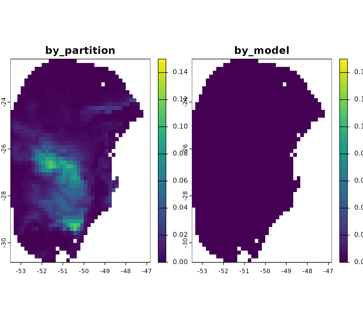
verbose = FALSE, overwrite = TRUE)The output is an object named variability_projections, a
list containing SpatRaster layers that represent the
variance deriving from replicates, models, and GCMs for each scenario
(including the present). These results can help detect areas where
prediction variability is higher.
For example, for the present time scenario, the variance mainly comes from differences among replicates.
In the most pessimistic scenario (SSP5-8.5) for 2081–2100, variability is not too high and comes primarily from replicates and GCMs.
# Variability for Future_2081-2100_ssp585
terra::plot(v$`Future_2081-2100_ssp585`, range = c(0, 0.1))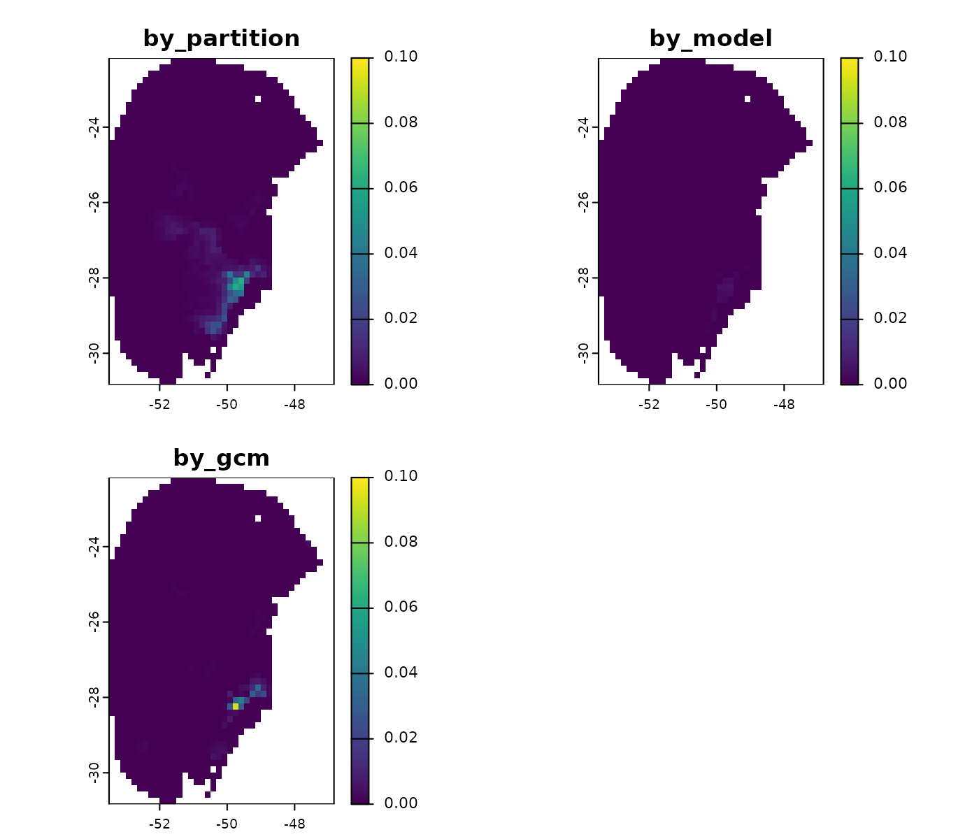
Importing Results
Because write_files = TRUE was set, the
variability_projections object includes the file path where
the results were saved. You can use this path with the
import_results() function to load the results when
needed.
# See the folder where the results were saved
v$root_directory
#> [1] "Temp/Projection_results/maxnet/variance"
As an example, we will import the results for the 2041–2060 period and the SSP1-2.6 scenario. In this scenario, the variability mainly originates from differences among the selected models (see below).
# Importing results
v_2041_2060_ssp126 <- import_results(projection = v,
                                     present = FALSE,  # Do not import results from the present time
                                     future_period = "2041-2060",
                                     future_pscen = "ssp126")

# Plot
terra::plot(v_2041_2060_ssp126, range = c(0, 0.1))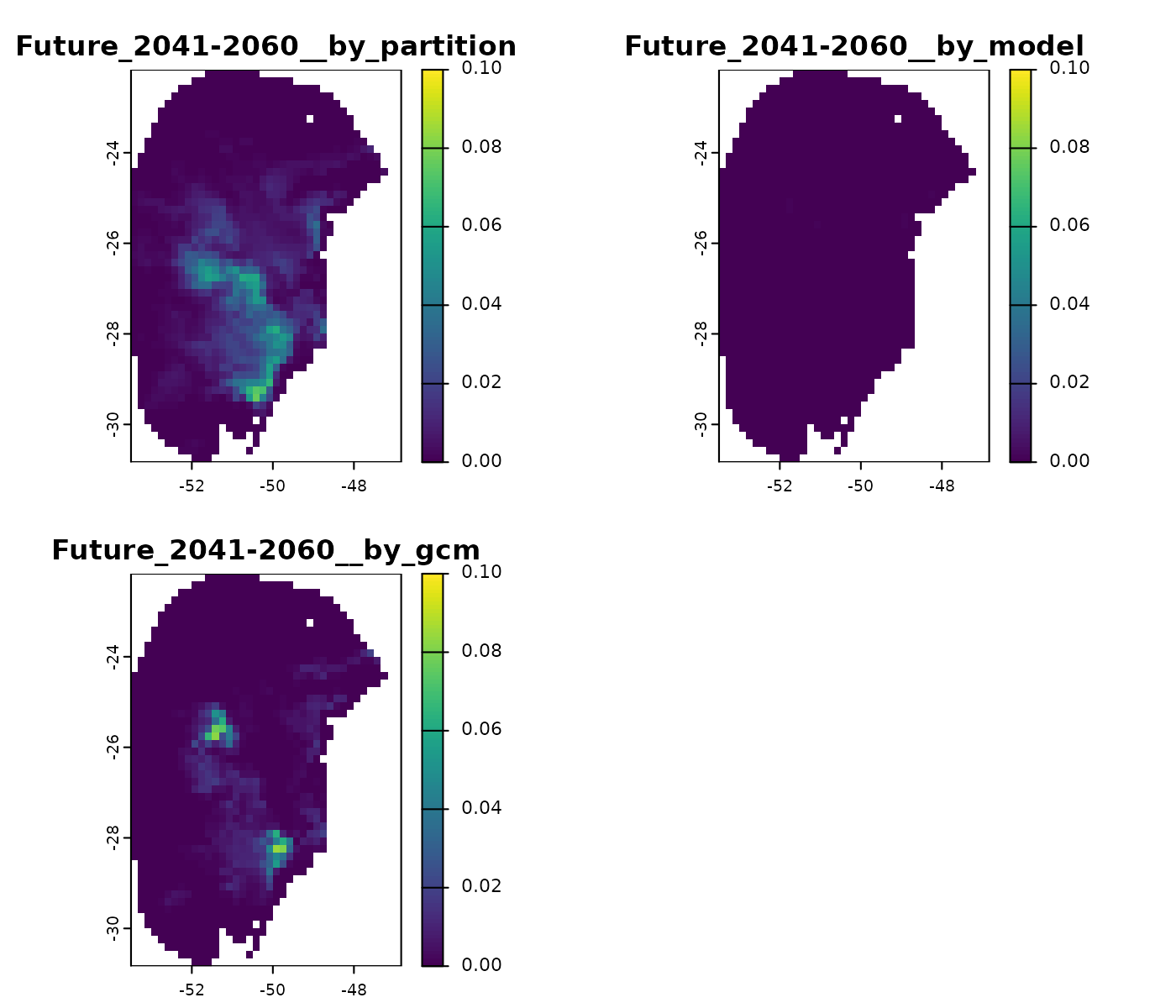
Saving results
The variability_projections object is a list that
contains resulting SpatRaster layers (if
return_raster = TRUE) and the directory path where the
results were saved (if write_files = TRUE).
If the results were not saved to disk during the initial run, you can
save the SpatRaster layers afterward using the
writeRaster() function. For example, to save the
variability map for one of the future scenarios:
writeRaster(v$`Future_2081-2100_ssp585`,
            file.path(out_dir, "Future_2081-2100_ssp585.tif"))
If the results were saved to disk, the
variability_projections object is automatically stored in a
folder named variance within the specified
output_dir. You can read this object to the R environment
in future sessions using the readRDS() function:
This object can then be used to import the results with the
import_results() function.
Assessing extrapolation risks
When projecting models to new regions or time periods, it is common to encounter conditions that are non-analogous to those used to train models.
For example, the maximum annual mean temperature (bio_1) in our model’s calibration data was :
max(fitted_model_maxnet$calibration_data$bio_1)
#> [1] 22.6858
In contrast, in future scenarios, conditions are projected to become warmer. To illustrate this, let’s import environmental variables from one of the GCMs (ACCESS-CM2) under the future scenario SSP5-8.5 and examine the maximum temperature:
# Import variables from the 2081-2100 period (SSP585, GCM MIROC6)
future_ACCESS_CM2 <- rast(file.path(out_dir_future,
                                "2081-2100/ssp585/ACCESS-CM2/Variables.tif"))

# Range of values in bio_1
terra::minmax(future_ACCESS_CM2$bio_1)
#>     bio_1
#> min  17.8
#> max  29.6

# Plot
terra::plot(future_ACCESS_CM2$bio_1,
            breaks = c(-Inf, 22.7, Inf))  # Highlight regions with values above 22.7ºC
Note that temperatures are expected to exceed the current maximum temperature in most of the area under future conditions.
The functions single_mop() and
projection_mop() compute the Mobility-Oriented Parity (MOP)
metric (Owens
et al. 2013) with recent updates implemented in the mop package (Cobos et al. 2024).
This metric calculates dissimilarity between training and projection
conditions, and detect areas with conditions outside training ranges.
Areas identified outside training ranges and those with large
dissimilarity (distances) values are where model predictions are a
product of extrapolation. Depending on how the model is predicting
outside ranges (see response curves), interpreting those results can be
risky because of uncertainties in prediction behavior (hence the term
extrapolation risks).
The MOP analysis requires the following inputs:
- Reference data: An object of class
fitted_modelsreturned by thefit_selected()function, or an object of classprepared_datareturned byprepare_data(). These objects contain the environmental data used during model training. - Data of interest for analysis:
- For
single_mop(), aSpatRasterwith the environmental variables representing a single scenario for model projections. - For
projection_mop(), an object of classprojection_datareturned by theprepare_projection()function, with the paths to raster layers representing environmental conditions of multiple scenarios for model projections.
- For
Important note: Most likely, MOP needs to consider only the variables
used in the selected models. For that reason, using a
fitted_models object and setting
subset_variables = TRUE is preferred.
By default, projection_mop() does not compute distances
and performs a basic type of MOP, which highlights only regions
with conditions outside training ranges. Alternatively, you can set:
-
type = "simple"to compute an additional layer with the number of variables with values outside training conditions per location. -
type = "detailed"to add multiple layers that identify exactly which variables exhibit conditions outside training ranges, and how. -
calculate_distance = TRUEto compute multivariate distances from training to all conditions in the scenarios of projections.
Below, we perform a detailed MOP to identify areas with extrapolation risk in the future scenarios for which predictions were made:
# Create a folder to save MOP results
out_dir_mop <- file.path(tempdir(), "MOPresults")
dir.create(out_dir_mop, recursive = TRUE)

# Run MOP
kmop <- projection_mop(data = fitted_model_maxnet, projection_data = pr,
                       subset_variables = TRUE,
                       calculate_distance = TRUE,
                       out_dir = out_dir_mop,
                       type = "detailed",
                       overwrite = TRUE, progress_bar = FALSE)
This application returns a mop_projections object, which
contains the paths to the directories where the results were saved. This
object can be used with the import_results() function to
load the results.
MOP result options
The results of the MOP analysis provide multiple perspectives on extrapolation risks. Each component a different aspect of the dissimilarity between training and projection environmental conditions.
When importing results, you can specify the periods and scenarios
(e.g., “2081-2100” and “ssp585”), as well as the type of MOP results to
load. By default, all available MOP types are imported, these include:
distances (if calculated), basic,
simple, towards_high_end,
towards_low_end, towards_high_combined, and
towards_low_combined.
Below, we explore all MOP results for the SSP5-8.5 scenario and the 2081–2100 period:
# Import results from MOP runs
mop_ssp585_2100 <- import_results(projection = kmop,
                                  future_period = "2081-2100",
                                  future_pscen = "ssp585")

# See types of results
names(mop_ssp585_2100)
#> [1] "distances"             "simple"                "basic"
#> [4] "towards_high_combined" "towards_low_combined"  "towards_high_end"
#> [7] "towards_low_end"
Distances
The element distances represents Euclidean or
Mahalanobis distances depending on what is defined in the argument
distance. Large distance values indicate greater
dissimilarity from training conditions, highlighting areas with high
extrapolation risk.
terra::plot(mop_ssp585_2100$distances)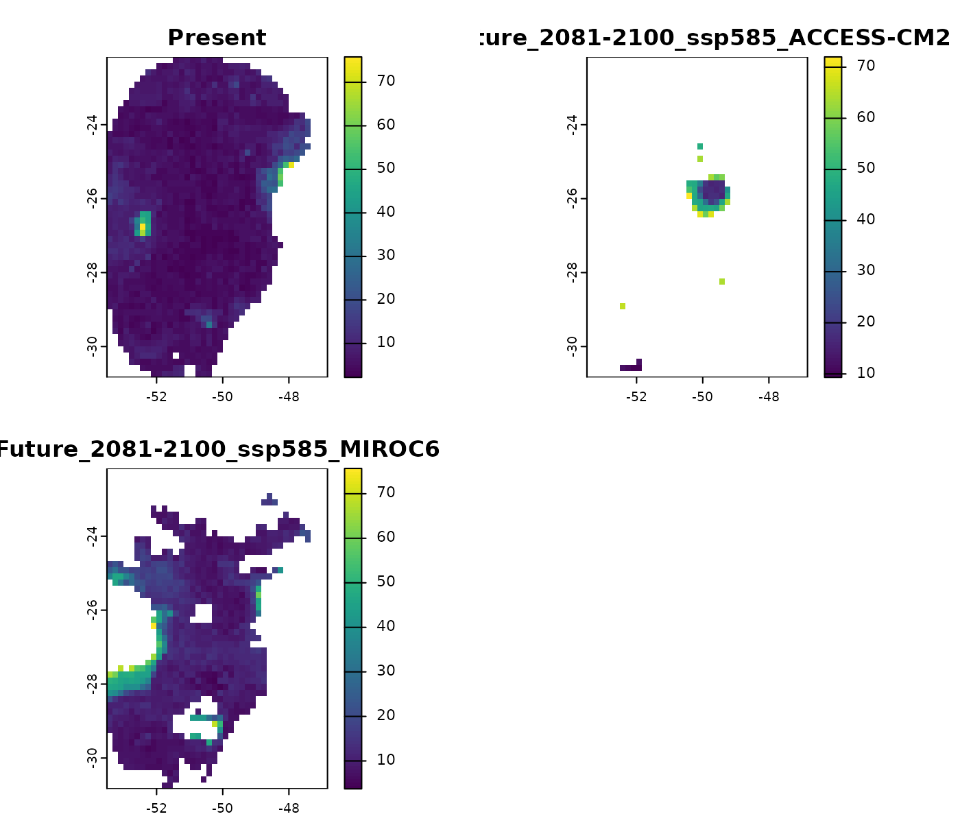
Basic
The element basic identifies areas where at least one
environmental variable is outside training conditions. A value of ‘1’
indicates the presence of non-analogous conditions in that specific area
and scenario.
terra::plot(mop_ssp585_2100$basic)
Simple
The results in simple quantify the number of
environmental variables in the projected area that outside training
conditions.
terra::plot(mop_ssp585_2100$simple)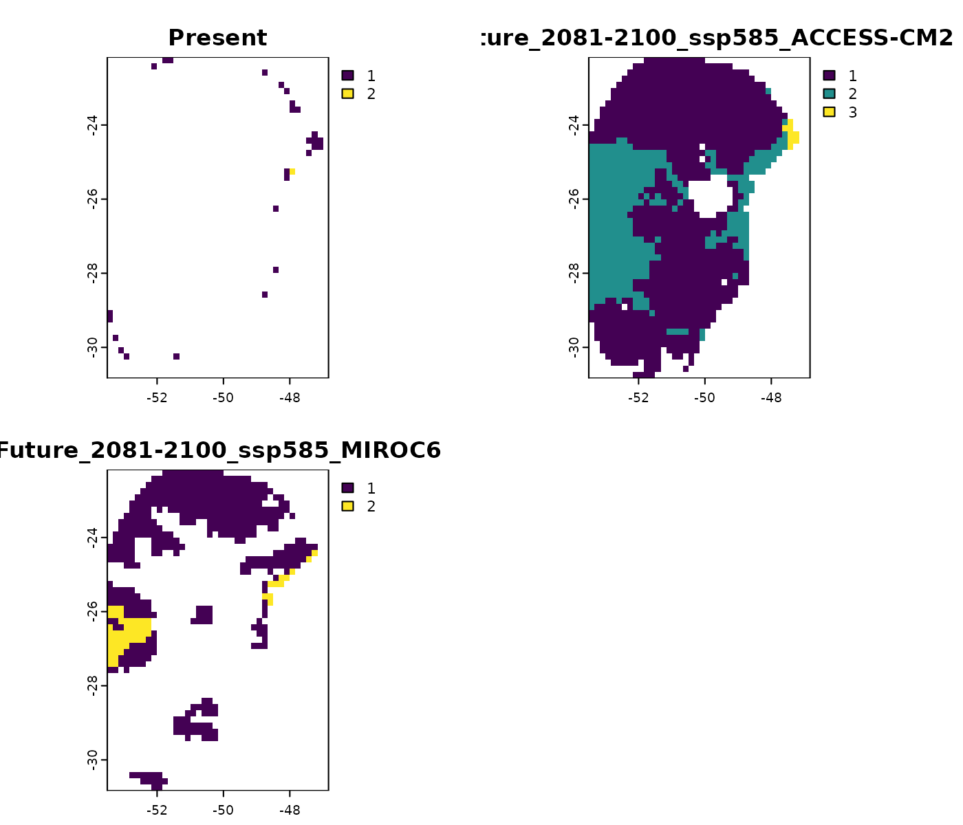
Towards high and low ends
The results in towards_high_end and
towards_low_end identify which areas show non-analogous
conditions for each of the variables independently. An important
detailed considered here is that the results show conditions above the
maximum (towards high) and below the minimum (towards low) values in
training data.
# Non-analogous conditions towards high values in the ACCESS-CM2 scenario
terra::plot(mop_ssp585_2100$towards_high_end$`Future_2081-2100_ssp585_ACCESS-CM2`)
# Non-analogous conditions towards low values in the MIROC6 scenario
terra::plot(mop_ssp585_2100$towards_low_end$`Future_2081-2100_ssp585_ACCESS-CM2`,
     main = names(mop_ssp585_2100$towards_low_end$`Future_2081-2100_ssp585_ACCESS-CM2`))
Combined results
The towards_high_combined and
towards_low_combined combine the previous results but keep
the identity of the variables detected outside ranges. Specifically,
towards_high_combined identifies variables with values
exceeding those observed in training data, whereas
towards_low_combined shows variables with values below the
training range.
# Variables with conditions above training range
terra::plot(mop_ssp585_2100$towards_high_combined)
# Variables with conditions below training range
terra::plot(mop_ssp585_2100$towards_low_combined)
Handling values within range
By default, the functions that run the MOP assign NA to
cells with values within the training range. Alternatively, you can
assign a value of 0 to these cells by setting
na_in_range = FALSE when running
projection_mop().
# Create a folder to save MOP results, now assigning 0 to cells within the range
out_dir_mop_zero <- file.path(tempdir(), "MOPresults_zero")
dir.create(out_dir_mop_zero, recursive = TRUE)

# Run MOP
kmop_zero <- projection_mop(data = fitted_model_maxnet, projection_data = pr,
                            subset_variables = TRUE,
                            na_in_range = FALSE,  # Assign 0 to cells within range
                            calculate_distance = TRUE,
                            out_dir = out_dir_mop_zero,
                            type = "detailed",
                            overwrite = TRUE, progress_bar = FALSE)
Let’s explore how this setting affects the simple and detailed MOP outputs:
# Import MOP for the scenario ssp585 in 2081-2100
mop_ssp585_2100_zero <- import_results(projection = kmop_zero,
                                       future_period = "2081-2100",
                                       future_pscen = "ssp585")

# Compare with the MOP that assigns NA to cells within the calibration range
# Simple MOP
terra::plot(c(mop_ssp585_2100$simple$`Future_2081-2100_ssp585_ACCESS-CM2`,
              mop_ssp585_2100_zero$simple$`Future_2081-2100_ssp585_ACCESS-CM2`),
            main = c("Within range as NA", "Within range as 0"))
# Detailed MOP
terra::plot(c(mop_ssp585_2100$towards_high_combined$`Future_2081-2100_ssp585_ACCESS-CM2`,
              mop_ssp585_2100_zero$towards_high_combined$`Future_2081-2100_ssp585_ACCESS-CM2`),
            main = c("Within range as NA", "Within range as 0"),
            plg=list(cex=0.6))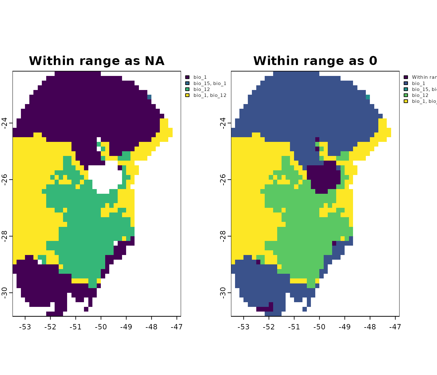
MOP results and response curves
While MOP helps us identify areas with non-analogous environmental conditions, whether risks of extrapolation exist depend on how model is behaving under non-analogous conditions. Model response curves are of great help to check model behavior under distinct conditions.
For example, consider a future scenario represented by the ACCESS-CM2 GCM and the SSP5-8.5 for 2081–2100. Here, values of bio_1 (Annual Mean Temperature), bio_12 (Annual Precipitation), and bio_15 (Precipitation Seasonality) exceed the upper limits observed in training data (see below).
# Non-analogous conditions towards high values in the ACCESS-CM2 scenario
terra::plot(mop_ssp585_2100$towards_high_combined$`Future_2081-2100_ssp585_ACCESS-CM2`)
Now, let’s check model response curves for these variables. To better
visualize how the model responds to environmental conditions in this
future scenario, we can set the plotting limits using this scenario’s
layers as new_data:
# Plotting response curves to check extrapolation towards the high end of variables
par(mfrow = c(1,3))  # Set plot grid
response_curve(models = fitted_model_maxnet, variable = "bio_1",
               new_data = future_ACCESS_CM2)
response_curve(models = fitted_model_maxnet, variable = "bio_12",
               new_data = future_ACCESS_CM2)
response_curve(models = fitted_model_maxnet, variable = "bio_15",
               new_data = future_ACCESS_CM2)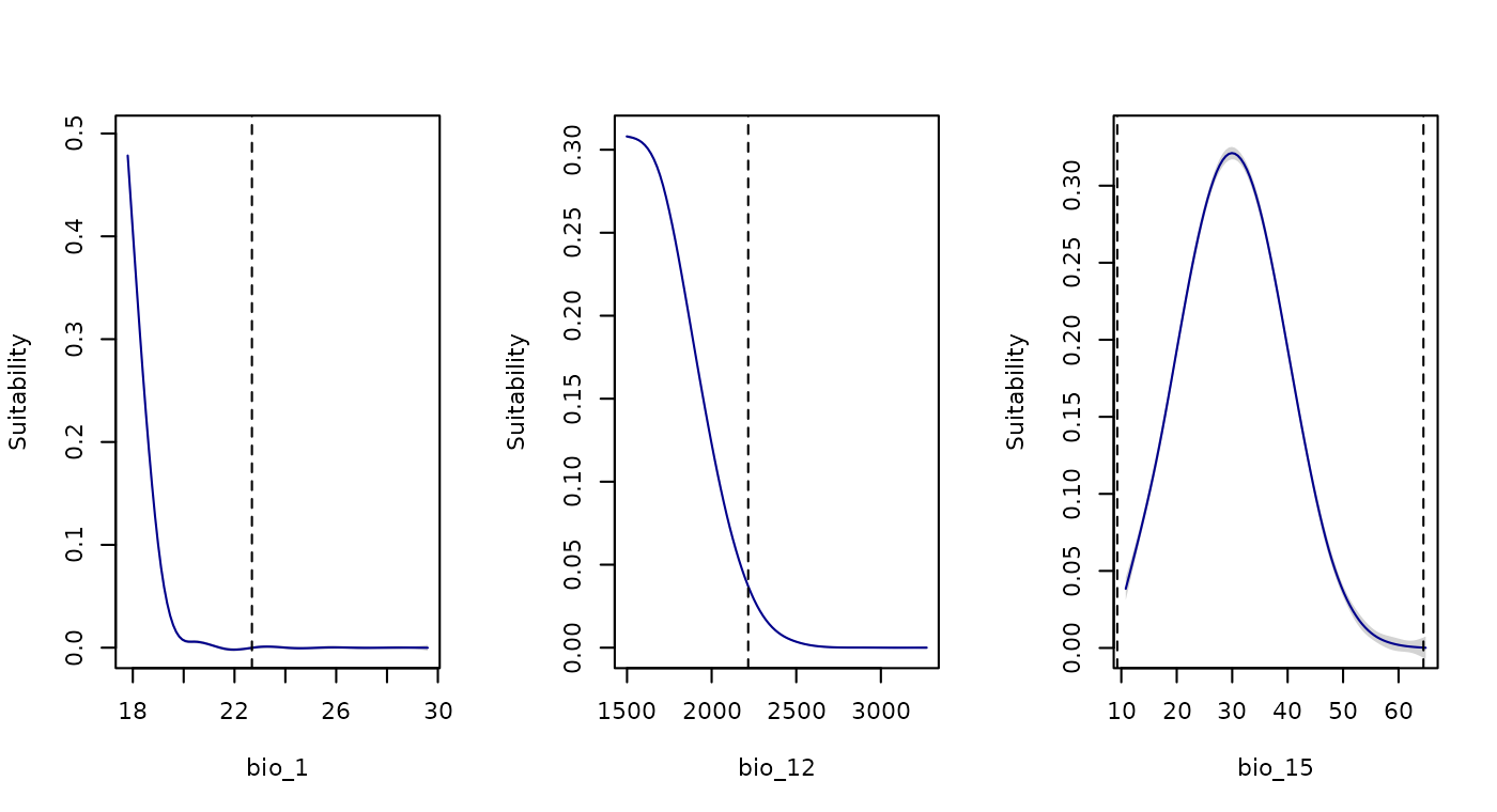
In the response curves for bio_1, bio_12, and bio_15, higher values correspond to lower suitability, reaching zero near the upper limit of training data (indicated by a dashed line). Beyond this upper limit, suitability remains close to zero, thus, we are not concerned about extrapolation risks towards higher values for these variables.
Next, let’s investigate the variables with values below the lower limit of training data:
# Non-analogous conditions towards low values in the ACCESS-CM2 scenario
par(mfrow = c(1, 2))  # Set grid
terra::plot(mop_ssp585_2100$towards_low_combined$`Future_2081-2100_ssp585_ACCESS-CM2`)

## It's bio 7. Plot response curve:
response_curve(models = fitted_model_maxnet, variable = "bio_7",
               new_data = future_ACCESS_CM2)
In some regions of the projection scenario, bio_7
(Temperature Annual Range) exhibits values below the lower limit of
the calibration data. The response curve indicates that suitability
continues to increase when extrapolating to these lower values. This is
a situation of concern due to extrapolation risks because we
are uncertain about when suitability should start to
decrease.
This example highlights why we strongly recommend interpreting MOP results alongside the response curves.
# Reset plotting parameters
par(original_par)
Saving and importing results
When projection_mop() is run, it automatically saves the
mop_projections object as an RDS file in
out_dir. You can load this object in R at any time using
the readRDS() function:
# Check for RDS files in the directory where we saved the MOP results
list.files(path = out_dir_mop, pattern = "rds")
#> [1] "mop_projections.rds"

# Import the mop_projections file
kmop <- readRDS(file.path(out_dir_mop, "mop_projections.rds"))