Import rasters resulting from projection functions
Source:R/import_projections.R
import_projections.RdThis function facilitates the import of rasters that have been generated and
written to disk by the project_selected(), projection_changes(),
variability_projections(), and projection_mop() functions. Users can
select specific periods (past/future), emission scenarios, General Circulation
Models (GCMs), and result types for import.
Usage
import_projections(
  projection,
  consensus = c("median", "range", "mean", "stdev"),
  present = TRUE,
  past_period = NULL,
  past_gcm = NULL,
  future_period = NULL,
  future_pscen = NULL,
  future_gcm = NULL,
  change_types = c("summary", "by_gcm", "by_change"),
  mop_types = c("distances", "simple", "basic", "towards_high_combined",
    "towards_low_combined", "towards_high_end", "towards_low_end")
)
Arguments
- projection
an object of class
model_projections,changes_projections,variability_projections, ormop_projections. This object is the direct output from one of the projection functions listed in the description.- consensus
(character) consensus measures to import. Available options are: 'median', 'range', 'mean' and 'stdev' (standard deviation). Default is c("median", "range", "mean", "stdev"), which imports all options. Only applicable if
projectionis amodel_projectionsobject.- present
(logical) wheter to import present-day projections. Default is TRUE. Not applicable if projection is a
changes_projectionsobject.- past_period
(character) names of specific past periods (e.g., 'LGM' or 'MID') to import. Default is NULL, meaning all available past periods will be imported.
- past_gcm
(character) names of specific General Circulation Models (GCMs) from the past to import. Default is NULL, meaning all available past GCMs will be imported.
- future_period
(character) names of specific future periods (e.g., '2041-2060' or '2081-2100') to import. Default is NULL, meaning all available future periods will be imported.
- future_pscen
(character) names of specific future emission scenarios (e.g., 'ssp126' or 'ssp585') to import. Default is NULL, meaning all available future scenarios will be imported.
- future_gcm
(character) names of specific General Circulation Models (GCMs) from the future to import. Default is NULL, meaning all available future GCMs will be imported.
- change_types
(character) names of the type of computed changes to import. Available options are: 'summary', 'by_gcm', 'by_change' and 'binarized'. Default is c("summary", "by_gcm", "by_change"), importing all types. Only applicable if projection is a
changes_projectionsobject.- mop_types
(character) type(s) of MOP to import. Available options are: 'basic', 'simple', 'towards_high_combined', 'towards_low_combined', towards_high_end', and 'towards_low_end'. Default is NULL, meaning all available MOPs will be imported. Only applicable if projection is a
mop_projectionsobject.
Value
A SpatRaster or a list of SpatRasters, structured according to the
input projection class:
If
projectionismodel_projections: A stackedSpatRastercontaining all selected projections.If
projectionischanges_projections: A list ofSpatRasters, organized by the selectedchange_types(e.g., 'summary', 'by_gcm', and/or 'by_change').If
projectionismop_projections: A list ofSpatRasters, organized by the selectedmop_types(e.g., 'simple' and 'basic').If
projectionisvariability_projections: A list ofSpatRasters, containing the computed variability.
Examples
# Load packages
library(terra)
#> terra 1.8.60
# Step 1: Organize variables for current projection
## Import current variables (used to fit models)
var <- terra::rast(system.file("extdata", "Current_variables.tif",
package = "kuenm2"))
## Create a folder in a temporary directory to copy the variables
out_dir_current <- file.path(tempdir(), "Current_raw2")
dir.create(out_dir_current, recursive = TRUE)
## Save current variables in temporary directory
terra::writeRaster(var, file.path(out_dir_current, "Variables.tif"))
# Step 2: Organize future climate variables (example with WorldClim)
## Directory containing the downloaded future climate variables (example)
in_dir <- system.file("extdata", package = "kuenm2")
## Create a folder in a temporary directory to copy the future variables
out_dir_future <- file.path(tempdir(), "Future_raw2")
## Organize and rename the future climate data (structured by year and GCM)
### 'SoilType' will be appended as a static variable in each scenario
organize_future_worldclim(input_dir = in_dir, output_dir = out_dir_future,
name_format = "bio_", fixed_variables = var$SoilType)
#>
|
| | 0%
|
|========= | 12%
|
|================== | 25%
|
|========================== | 38%
|
|=================================== | 50%
|
|============================================ | 62%
|
|==================================================== | 75%
|
|============================================================= | 88%
|
|======================================================================| 100%
#>
#> Variables successfully organized in directory:
#> /tmp/Rtmphkhpn9/Future_raw2
# Step 3: Prepare data to run multiple projections
## An example with maxnet models
## Import example of fitted_models (output of fit_selected())
data(fitted_model_maxnet, package = "kuenm2")
## Prepare projection data using fitted models to check variables
pr <- prepare_projection(models = fitted_model_maxnet,
present_dir = out_dir_current,
future_dir = out_dir_future,
future_period = "2041-2060",
future_pscen = c("ssp126", "ssp585"),
future_gcm = c("ACCESS-CM2", "MIROC6"),
raster_pattern = ".tif*")
# Step 4: Run multiple model projections
## A folder to save projection results
out_dir <- file.path(tempdir(), "Projection_results/maxnet")
dir.create(out_dir, recursive = TRUE)
## Project selected models to multiple scenarios
p <- project_selected(models = fitted_model_maxnet, projection_data = pr,
out_dir = out_dir)
#>
|
| | 0%
|
|============== | 20%
|
|============================ | 40%
|
|========================================== | 60%
|
|======================================================== | 80%
|
|======================================================================| 100%
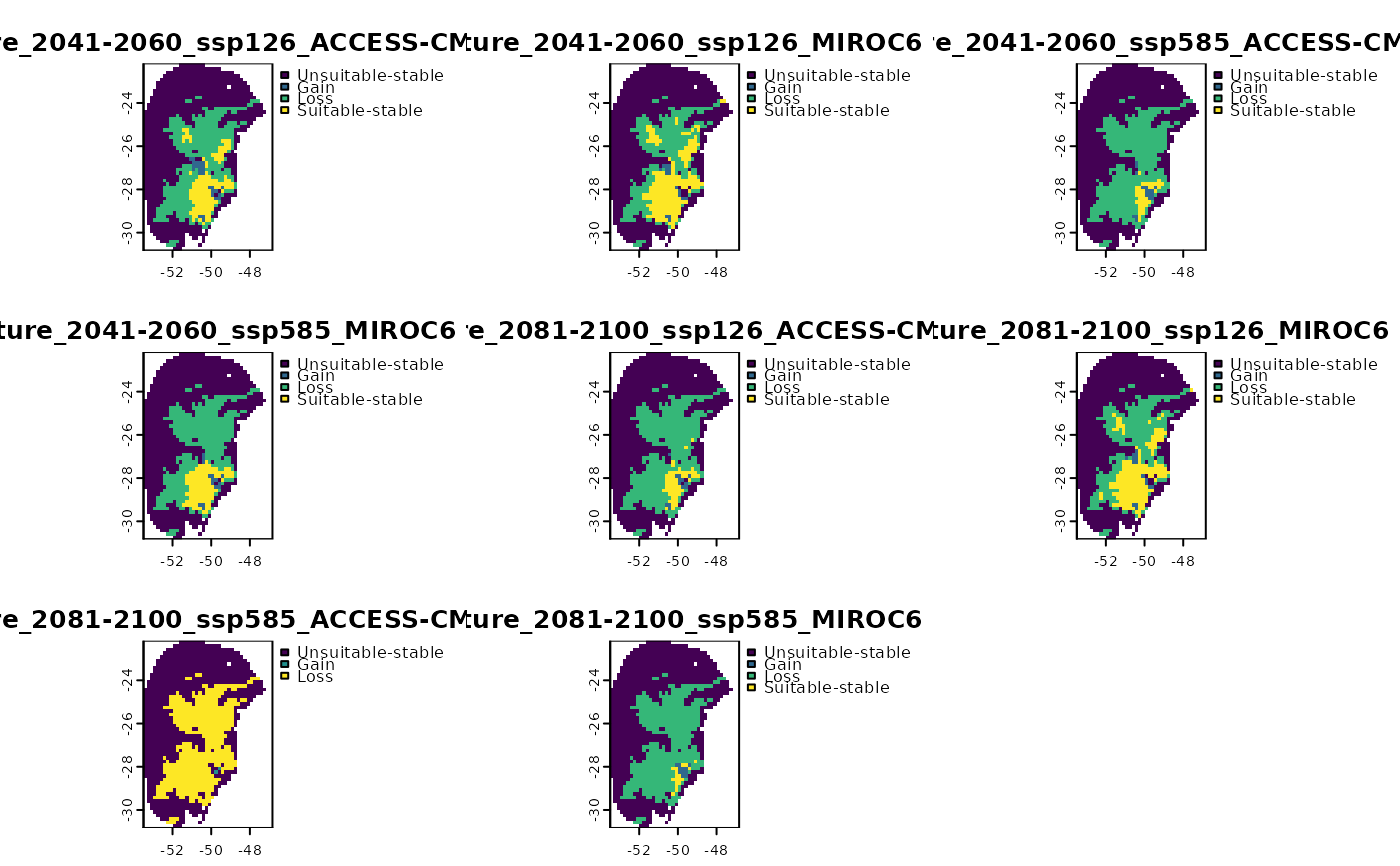
# Use import_projections to import results:
raster_p <- import_projections(projection = p, consensus = "mean")
plot(raster_p)