Summary
- Description
- Getting ready
- Fitting selected models
- Response curves
- Variable importance
- Evaluation with independent data
- Saving a fitted_models object
Description
After the best performing models have been selected, users need to
fit this models (using fit_selected()) in order to explore
their characteristics and continue with the next steps. Fitted models
can then be used to assess variable importance in models, as well as to
explore variable response curves. Selected models can also be evaluated
using independent records that were not used during calibration. This
vignette contains examples to explore the multiple options available to
fit and explore selected models.
Getting ready
At this point it is assumed that kuenm2 is installed (if
not, see the Main
guide). Load kuenm2 and any other required packages,
and define a working directory (if needed).
Note: functions from other packages (i.e., not from base R or
kuenm2) used in this guide will be displayed as
package::function().
# Load packages
library(kuenm2)
library(terra)

# Current directory
getwd()

# Define new directory
#setwd("YOUR/DIRECTORY")  # uncomment and modify if setting a new directory

# Saving original plotting parameters
original_par <- par(no.readonly = TRUE)
Fitting selected models
To fit the selected models, we need a
calibration_results object. For more details in model
calibration, please refer to the vignette Model Calibration. The
calibration_results object generated in this vignette is
available as a data example in the package. Let’s load it.
# Import an example of calibration results
data("calib_results_maxnet", package = "kuenm2")

# Print calibration result
calib_results_maxnet
#> calibration_results object summary (maxnet)
#> =============================================================
#> Species: Myrcia hatschbachii
#> Number of candidate models: 300
#>   - Models removed because they failed to fit: 0
#>   - Models identified with concave curves: 39
#>   - Model with concave curves not removed
#>   - Models removed with non-significant values of pROC: 0
#>   - Models removed with omission error > 10%: 165
#>   - Models removed with delta AIC > 2: 133
#> Selected models: 2
#>   - Up to 5 printed here:
#>      ID
#> 192 192
#> 219 219
#>                                                                                      Formulas
#> 192                        ~bio_1 + bio_7 + bio_15 + I(bio_1^2) + I(bio_7^2) + I(bio_15^2) -1
#> 219 ~bio_1 + bio_7 + bio_12 + bio_15 + I(bio_1^2) + I(bio_7^2) + I(bio_12^2) + I(bio_15^2) -1
#>     Features R_multiplier pval_pROC_at_10.mean Omission_rate_at_10.mean
#> 192       lq          0.1                    0                   0.0769
#> 219       lq          0.1                    0                   0.0962
#>         dAIC Parameters
#> 192 0.000000          6
#> 219 1.179293          7
This object contains the results of candidate models calibrated using
the maxnet algorithm. The package also provides a similar
example wit models created using the glm algorithm. See
below how to load the calib_results_glm object in case you
want to explore it.
# Import calib_results_glm
data("calib_results_glm", package = "kuenm2")

# Print calibration result
calib_results_glm
#> calibration_results object summary (glm)
#> =============================================================
#> Species: Myrcia hatschbachii
#> Number of candidate models: 122
#>   - Models removed because they failed to fit: 0
#>   - Models identified with concave curves: 18
#>   - Model with concave curves not removed
#>   - Models removed with non-significant values of pROC: 0
#>   - Models removed with omission error > 10%: 101
#>   - Models removed with delta AIC > 2: 20
#> Selected models: 1
#>   - Up to 5 printed here:
#>    ID                                                        Formulas Features
#> 85 85 ~bio_1 + bio_7 + bio_12 + I(bio_1^2) + I(bio_7^2) + I(bio_12^2)       lq
#>    pval_pROC_at_10.mean Omission_rate_at_10.mean dAIC Parameters
#> 85                    0                   0.0904    0          6
Note that the calibration_results object stores only the
information related to the calibration process and model evaluation, it
does not include the fitted maxnet (or glm)
models.
To obtain fitted models, we need to use the
fit_selected() function. By default, this function fits a
full model (i.e., without replicates and without splitting the data into
training and testing sets). However, you can configure it to fit final
models with replicates if desired.
In this example, we’ll fit the final models with 4 k-fold replicates (leaving one fold out), as in the Model Calibration vignette.
# Fit selected models using calibration results
fm <- fit_selected(calibration_results = calib_results_maxnet,
                   replicate_method = "kfolds", n_replicates = 4)
# Fitting replicates...
#   |========================================================================| 100%
# Fitting full models...
#   |========================================================================| 100%
The fit_selected() function returns a
fitted_models object, a list that contains essential
information from the fitted models, which is required for the subsequent
steps.
You can explore the contents of the fitted_models object
by indexing its elements. For example, the fitted maxnet
(or glm) model objects are stored within the
Models element. Note that Models is a nested
list: for each selected model (in this case, models 192 and 219), it
includes both the replicates (if fitted with replicates) and the full
model.
# See names of selected models
names(fm$Models)
#> [1] "Model_192" "Model_219"

# See models inside Model 192
names(fm$Models$Model_192)
#> [1] "Replicate_1" "Replicate_2" "Replicate_3" "Replicate_4" "Full_model"
The fitted_models object also stores the thresholds that
can be used to binarize the models into suitable and unsuitable areas.
These thresholds correspond to the omission error used during model
selection (e.g., 5% or 10%).
You can access the omission error used to calculate the thresholds directly from the object:
# Get omission error used to select models and calculate the theshold values
fm$omission_rate
#> [1] 10
The omission error used to calculate the thresholds was 10%, meaning that when the predictions are binarized, approximately 10% of the presence records used to calibrate the models will fall into cells with predicted values below the threshold.
The thresholds are summarized in two ways: the mean and median across replicates for each model, and the consensus mean and median across all selected models (when more than one model is selected):
fm$thresholds
#> $Model_192
#> $Model_192$mean
#> [1] 0.2449115
#>
#> $Model_192$median
#> [1] 0.266498
#>
#>
#> $Model_219
#> $Model_219$mean
#> [1] 0.260294
#>
#> $Model_219$median
#> [1] 0.2695625
#>
#>
#> $consensus
#> $consensus$mean
#> [1] 0.2526028
#>
#> $consensus$median
#> [1] 0.2674515
#>
#>
#> $type
#> [1] "cloglog"
Response curves
The selected models in the fitted_models object can be
used to generate response curves. Individual variable response curves
illustrate how each environmental variables influences suitability,
while keeping all other variables constant.
By default, the curves are generated with all other variables set to
their mean values (or the mode for categorical variables). The mean or
mode are calculated from the combined set of presence and background
data (averages_from = "pr_bg"). You can change this
behavior to use only the presence localities by setting
averages_from = "pr".
All response curves
An easy way to explore response curves for all variables is as follows:
# Produce response curves for all variables in all fitted models
all_response_curves(fm)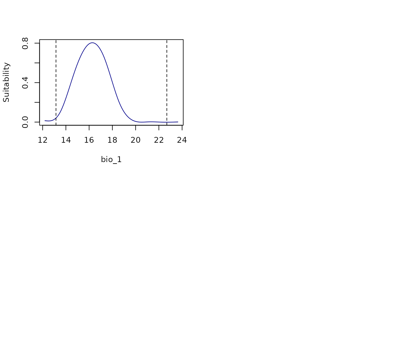
In the previous plot, the dashed lines indicate the range of
variables values in the data used to fit models. If multiple models were
fitted, variability is shown via a Generalized Additive Model (GAM)
using the mean and the 95% confidence interval. For a more detailed view
of what the response curve for each of the models fitted look like, the
argument show_lines can be set to TRUE.
# All response curves showing each model as a different line
all_response_curves(fm, show_lines = TRUE)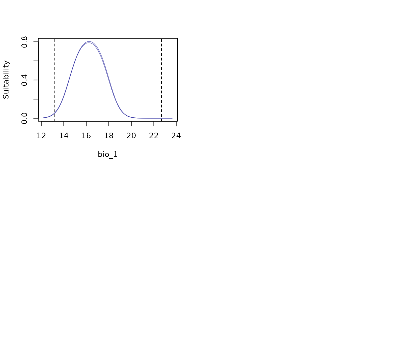
To explore response curves of all variables for each model
independently, the argument model_ID can be used. The plot
will show variable response curves for the full model.
# All response curves for model 219
all_response_curves(fm, modelID = "Model_219")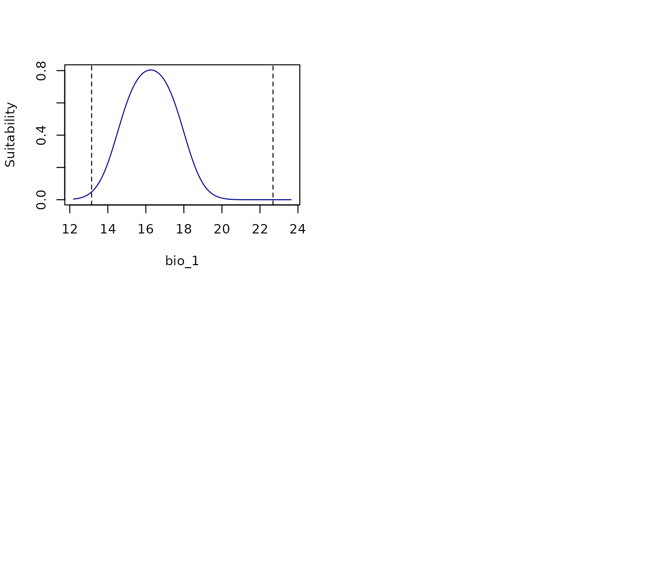
To get a view of variability in response curves for a model produced
with replicates, use show_variability = TRUE. Both, the GAM
or the multiple-line approaches can be used to show variability.
# All response curves for model 219 (GAM for variability)
all_response_curves(fm, modelID = "Model_219", show_variability = TRUE)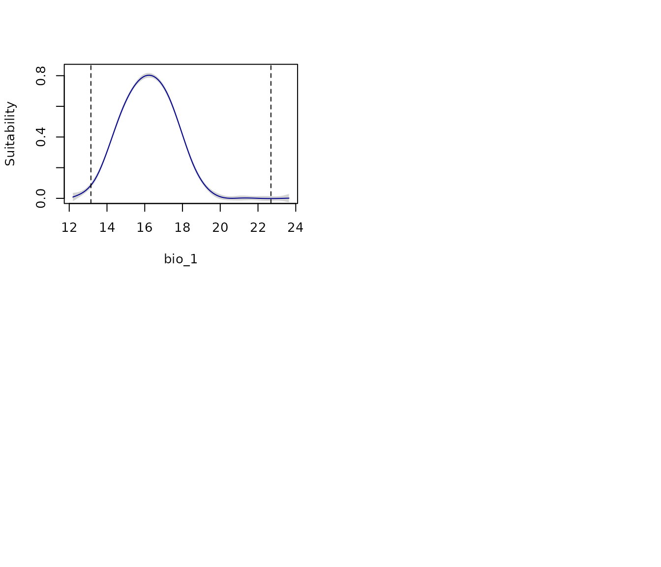
# All response curves for model 219 (each curve is a replicate)
all_response_curves(fm, modelID = "Model_219", show_variability = TRUE,
                    show_lines = TRUE)
Customized response curves
The previous plots help to gain a quick understanding of response curves for fitted models, but little can be done make each panel look better. To produce nicer plots, response curves for each variable at a time can be produced. Let’s check which variables are available to plot by examining the coefficients of the full models:
# Get variables with non-zero coefficients in the models
fm$Models[[1]]$Full_model$betas  # From the first model selected
#>        bio_1        bio_7       bio_15   I(bio_1^2)   I(bio_7^2)  I(bio_15^2)
#> 11.572321659  0.215970079  0.369077970 -0.356605446 -0.020306099 -0.006200151
fm$Models[[2]]$Full_model$betas  # From the second model selected
#>         bio_1        bio_12        bio_15    I(bio_1^2)    I(bio_7^2)
#>  1.178814e+01  1.638570e-02  3.406100e-01 -3.625405e-01 -1.440450e-02
#>   I(bio_12^2)   I(bio_15^2)
#> -5.261860e-06 -5.623987e-03
The variables bio_1, bio_7,
bio_12 and bio_15have non-zero coefficient
values, which means they contribute to the model and are available for
generating response curves.
Remember that response curves are computed using all selected models. This time let’s change the margins and labels for each plot
par(mfrow = c(2, 2), mar = c(4, 4, 1, 0.5))  # Set grid of plot
response_curve(models = fm, variable = "bio_1", las = 1)
response_curve(models = fm, variable = "bio_7", ylab = "", las = 1)
response_curve(models = fm, variable = "bio_12", las = 1)
response_curve(models = fm, variable = "bio_15", ylab = "", las = 1)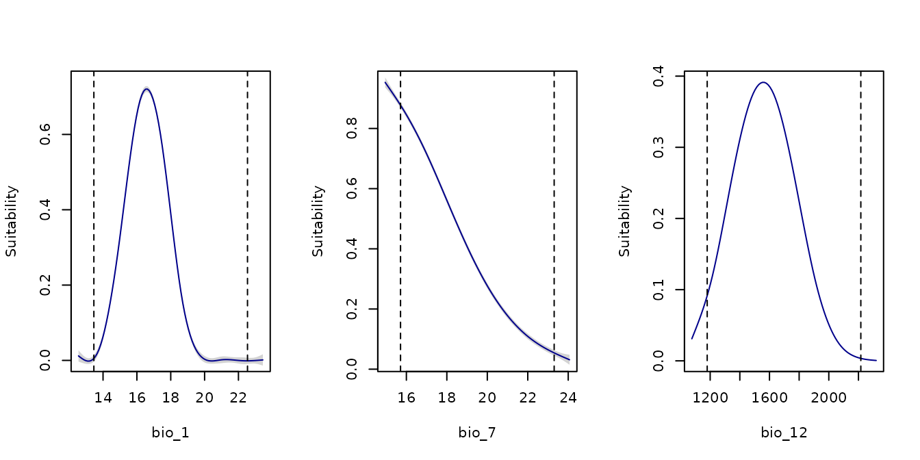
We can also specify which of the selected models should be used to generate the response curves:
par(mfrow = c(2, 2), mar = c(4, 4, 2.5, 0.5))  # Set grid of plot
response_curve(models = fm, variable = "bio_1", modelID = "Model_192",
               main = "Model_192", las = 1)
response_curve(models = fm, variable = "bio_1", modelID = "Model_219",
               main = "Model_219", ylab = "", las = 1)
response_curve(models = fm, variable = "bio_7", modelID = "Model_192",
               main = "Model_192", las = 1)
response_curve(models = fm, variable = "bio_7", modelID = "Model_219",
               main = "Model_219", ylab = "", las = 1)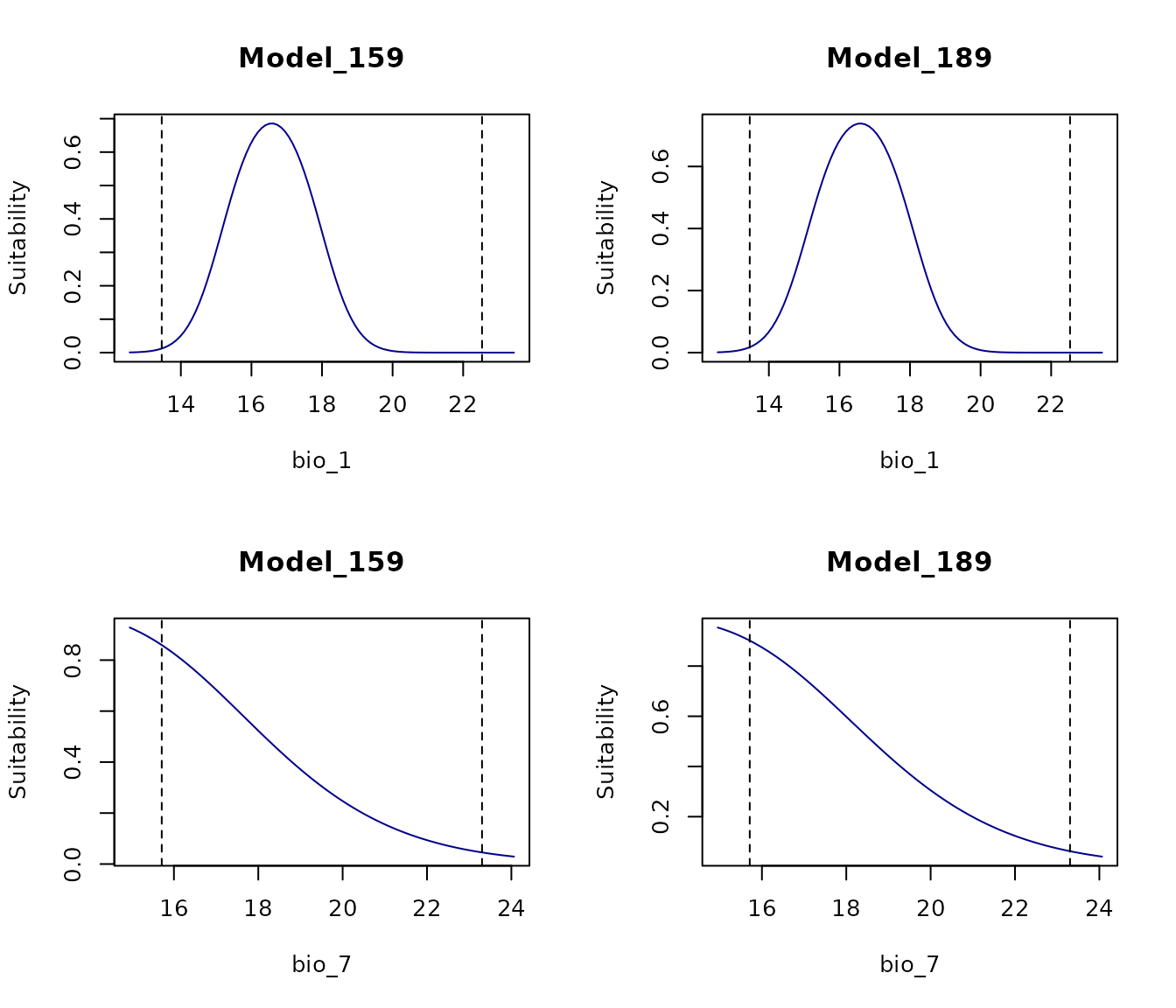
By default, the response curve extends beyond the range of model
fitting limits (dashed lines) based on the observed range of values and
an extrapolation_factor (when
extrapolation = TRUE). The default extrapolation factor is
set to 10% of the range.
If extrapolation = FALSE, no extrapolation occurs, and
the plot limits match the fitting data range exactly.
We can increase the extrapolation factor to allow a broader range beyond the observed data. Below is the response curve plotted with an extrapolation factor of 2:
par(mfrow = c(2, 2), mar = c(4, 4, 1, 0.5))  # Set grid of plot
response_curve(models = fm, variable = "bio_1", extrapolation_factor = 2,
               las = 1)
response_curve(models = fm, variable = "bio_7", extrapolation_factor = 2,
               ylab = "", las = 1)
response_curve(models = fm, variable = "bio_12", extrapolation_factor = 2,
               las = 1)
response_curve(models = fm, variable = "bio_15", extrapolation_factor = 2,
               ylab = "", las = 1)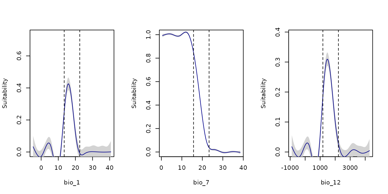
Note that the response curve now extends further beyond the observed
data range. Optionally, we can manually set the lower and upper limits
of the variables. For example, since bio_12 represents
annual precipitation and negative values are not realistic, we can set
its lower limit to 0:
response_curve(models = fm, variable = "bio_12", extrapolation_factor = 0.1,
               l_limit = 0)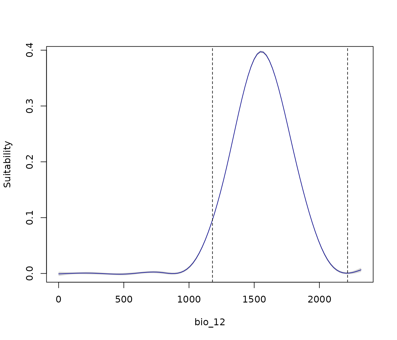
Now, the lower limit of the plot for bio_12 is set to 0.
Since we did not specify an upper limit, the plot uses the extrapolation
factor (here, 0.1) to define the upper limit.
The other aspect to notice after increasing the extrapolation factor
is that the curves looked like they were not perfectly unimodal.
Unfortunately, using a GAM to summarize and represent variability can
some times generate this effect. However, plotting responses for each
model as independent curves will show the real shape of the curve, see
the differences after setting show_lines = TRUE.
par(mfrow = c(1, 2), mar = c(4, 4, 1, 0.5))  # Set grid of plot
response_curve(models = fm, variable = "bio_1", extrapolation_factor = 0.5,
               las = 1)
response_curve(models = fm, variable = "bio_1", extrapolation_factor = 0.5,
               show_lines = TRUE, ylab = "", las = 1)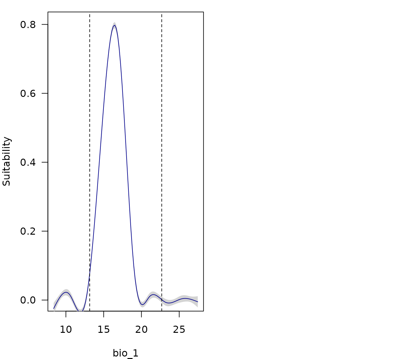
Optionally, we can add the presence and background points used to fit
the models to the response curve plot by setting
add_points = TRUE:
response_curve(models = fm, variable = "bio_1", show_lines = TRUE,
               add_points = TRUE)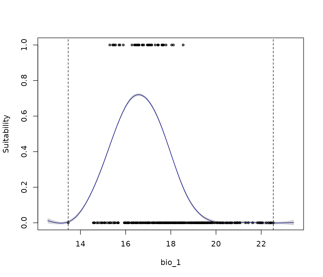
Bivariate response curves
All previous curve plots are showing responses to individual variables. Exploring responses to two variables at a time can help understand the small differences between models fitted with distinct terms. Let’s see an example below:
# First, let's check the terms in the models fitted
## Model 192
fm$Models$Model_192$Full_model$betas
#>        bio_1        bio_7       bio_15   I(bio_1^2)   I(bio_7^2)  I(bio_15^2)
#> 11.572321659  0.215970079  0.369077970 -0.356605446 -0.020306099 -0.006200151

## Model 219
fm$Models$Model_219$Full_model$betas
#>         bio_1        bio_12        bio_15    I(bio_1^2)    I(bio_7^2)
#>  1.178814e+01  1.638570e-02  3.406100e-01 -3.625405e-01 -1.440450e-02
#>   I(bio_12^2)   I(bio_15^2)
#> -5.261860e-06 -5.623987e-03

# Example of a bivariate response plot
bivariate_response(models = fm, variable1 = "bio_1", variable2 = "bio_15",
                   modelID = "Model_192")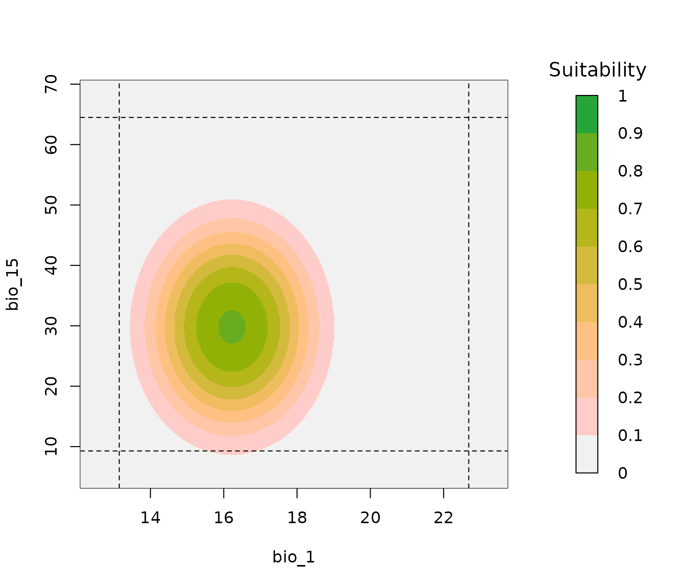
In the previous plot, the dashed lines represent the limits of the data used for model fitting, and darker colors represent higher suitability. Let’s now compare the two models and check if there are any differences. Multiple bivariate response plots can be put together in a single plot if the suitability bar legend is not used.
par(mfrow = c(1, 2), mar = c(4, 4, 2.5, 0.5))

# Bivariate response model 192
bivariate_response(models = fm, variable1 = "bio_1", variable2 = "bio_15",
                   modelID = "Model_192", add_bar = FALSE, main = "Model 192")

# Bivariate response model 219
bivariate_response(models = fm, variable1 = "bio_1", variable2 = "bio_15",
                   modelID = "Model_219", add_bar = FALSE, main = "Model 219",
                   ylab = "")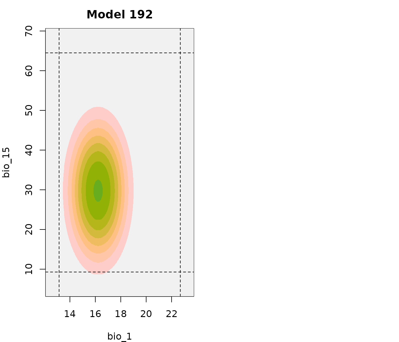
These two models look very similar, the only noticeable difference is that suitability values above the threshold extend farther on variable bio_15 for model 219. More noticeable effects can be seen in bivariate representations when fitted models include or not product terms. However, as in this example, even a small variation on the number or type of terms included in a model can change how predictions look like.
Variable importance
The relative importance of model predictors can be calculated
exploring the deviance using the var_importance() function.
This process starts by fitting the full model (maxnet or
glm), which includes all predictors. Then, the function
fits separate models excluding one predictor at a time, and quantifies
how the removal affects model performance. The values of contribution
are computed for variables by default, but explorations by terms are
also possible using the argument by_terms (i.e., if the
model includes linear and quadratic terms of a variable, the process
will run for each of them separately).
By default, the function runs on a single core. You can enable
parallel processing by setting parallel = TRUE and
specifying the number of cores with ncores. Note that
parallelization only speeds up the computation when there are many
variables (e.g., >17) and the calibration dataset is large (e.g.,
over 15,000 total points).
Variable importance is computed for all selected models by default:
# Calculate variable importance
imp <- variable_importance(models = fm)

# Calculating variable contribution for model 1 of 2
#   |======================================================================| 100%
# Calculating variable contribution for model 2 of 2
#   |======================================================================| 100%
The function returns a data.frame with the relative
contribution of each variable. If multiple models are included in the
fitted object, an additional column identifies each
model.
imp
#>   predictor contribution    Models
#> 1     bio_1  0.567815429 Model_192
#> 2    bio_15  0.219231619 Model_192
#> 3     bio_7  0.212952953 Model_192
#> 4     bio_1  0.721574882 Model_219
#> 5    bio_15  0.248819713 Model_219
#> 6    bio_12  0.025950948 Model_219
#> 7     bio_7  0.003654457 Model_219
We can visualize variable importance using the
plot_importance() function. When the
fitted_models object contains more than one selected model,
contributions are displayed as a boxplot, along with the mean
contribution, and the number (N) of fitted models with that
predictor.
plot_importance(imp)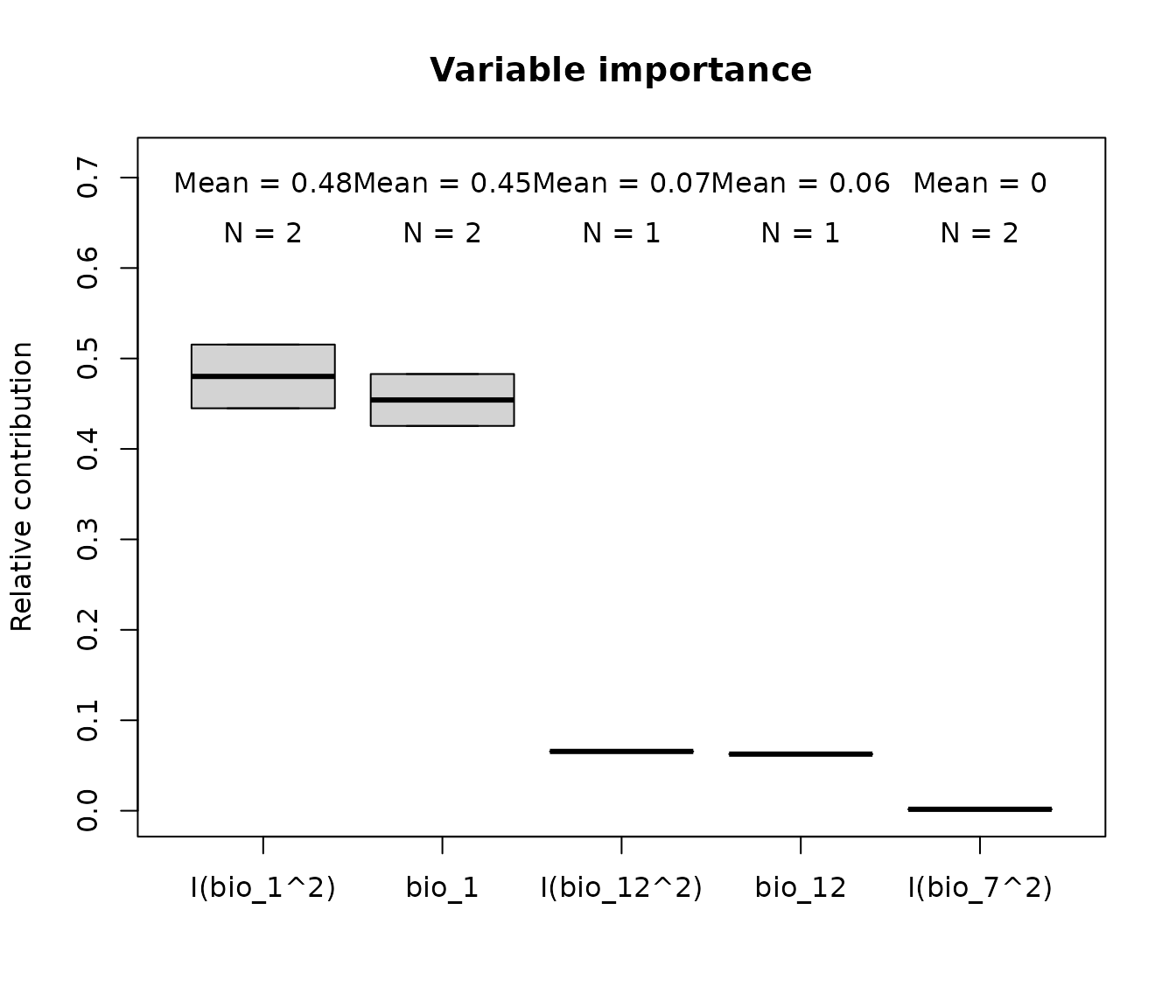
If variable importance is computed for a single model, the plot displays a bars instead of boxes:
# Calculate variable importance for a specific selected Model
imp_192 <- variable_importance(models = fm, modelID = "Model_192",
                               progress_bar = FALSE)

# Plot variable contribution for model 192
plot_importance(imp_192, main = "Variable importance: Model 192")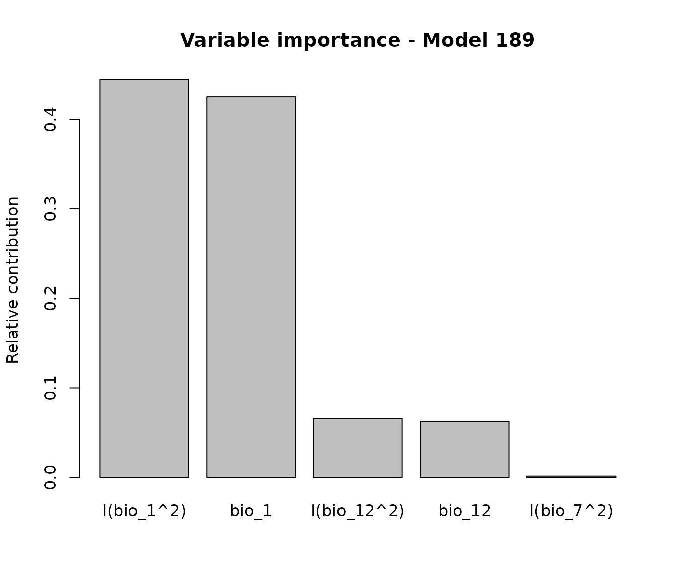
The previous examples show how important are variables by checking
the change in models if we remove a variable completely from the
equation. To compute contribution of all variable terms (i.e., how
important is to keep distinct terms of the same variable) set
by_terms = TRUE:
# Calculate variable importance for a specific selected Model
imp_terms <- variable_importance(models = fm, by_terms = TRUE,
                                 progress_bar = FALSE)
#>
#> Calculating variable contribution for model 1 of 2
#>
#> Calculating variable contribution for model 2 of 2

# Check results
imp_terms
#>      predictor contribution    Models
#> 1   I(bio_1^2)  0.330546900 Model_192
#> 2        bio_1  0.295001412 Model_192
#> 3       bio_15  0.209668355 Model_192
#> 4  I(bio_15^2)  0.156926301 Model_192
#> 5   I(bio_7^2)  0.006279520 Model_192
#> 6        bio_7  0.001577512 Model_192
#> 7   I(bio_1^2)  0.368476226 Model_219
#> 8        bio_1  0.332782286 Model_219
#> 9       bio_15  0.155708606 Model_219
#> 10 I(bio_15^2)  0.095186390 Model_219
#> 11 I(bio_12^2)  0.022722557 Model_219
#> 12      bio_12  0.021793617 Model_219
#> 13  I(bio_7^2)  0.003330318 Model_219

# Plot variable contribution for model 192
par(cex = 0.7, mar = c(3, 4, 2.5, 0.5))  # Set grid of plot
plot_importance(imp_terms, main = "Importance of variable terms")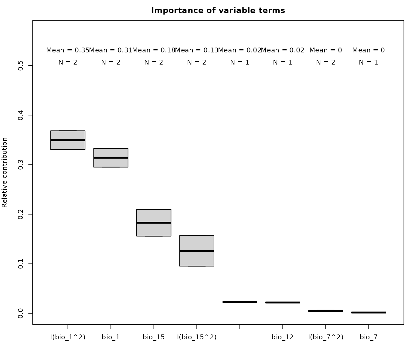
Evaluation with independent data
Selected models can be evaluated using an independent set of presence records (not used when fitting selected models). This approach is especially useful when new records become available. This can be useful to assess models for invasive species, for which model fitting is usually done in native areas with transfers to potential invasive areas.
The independent_evaluation() function computes omission
rates (i.e., the proportion of independent records predicted as below
the suitability threshold) and partial ROC. The function also assesses
whether environmental conditions in independent data are analogous those
under which models were fit using the mobility oriented-parity metric
(MOP; Cobos
et al. 2024).
Let’s use the new_occ as an example of independent data
(provided in the package). This dataset contains coordinates of
Myrcia hatschbachii sourced from NeotropicTree (Oliveira-Filho, 2017), and they
were not part of the data used to fit the models.
# Import independent records
data("new_occ", package = "kuenm2")

# See data structure
str(new_occ)
#> Classes 'data.table' and 'data.frame':   82 obs. of  3 variables:
#>  $ species: chr  "Myrcia hatschbachii" "Myrcia hatschbachii" "Myrcia hatschbachii" "Myrcia hatschbachii" ...
#>  $ x      : num  -48.3 -49.1 -49.9 -49.4 -49.9 ...
#>  $ y      : num  -25.2 -25 -24.5 -24.5 -24.8 ...
#>  - attr(*, ".internal.selfref")=<pointer: (nil)>
In order to evaluate predictive ability of models and how analogous
conditions in independent data are to fitting conditions, environmental
values need to be extracted to these new records. Let’s import the
raster variables and extract values for new_occ:
# Import raster layers
var <- terra::rast(system.file("extdata", "Current_variables.tif",
                               package = "kuenm2"))

# Extract variables to occurrences
new_data <- extract_occurrence_variables(occ = new_occ, x = "x", y = "y",
                                         raster_variables = var)

# See data structure
str(new_data)
#> 'data.frame':    82 obs. of  8 variables:
#>  $ pr_bg   : num  1 1 1 1 1 1 1 1 1 1 ...
#>  $ x       : num  -48.3 -49.1 -49.9 -49.4 -49.9 ...
#>  $ y       : num  -25.2 -25 -24.5 -24.5 -24.8 ...
#>  $ bio_1   : num  20.2 18 16.6 17.8 16.7 ...
#>  $ bio_7   : num  16.7 18.2 19.9 19.4 20.1 ...
#>  $ bio_12  : num  2015 1456 1526 1414 1578 ...
#>  $ bio_15  : num  43.8 33.7 29.1 32.2 26.5 ...
#>  $ SoilType: num  6 6 6 6 6 10 10 10 10 10 ...
Finding non-analogous conditions in independent records is not uncommon, especially in regions outside model calibration areas. To better illustrate this case, let’s add three fake records, in which some variables have non-analogous values, either higher than the upper limit or lower than the lower limit observed in the data used to fit models.
# Add some fake data beyond the limits of calibration ranges
fake_data <- data.frame("pr_bg" = c(1, 1, 1),
                        "x" = c(NA, NA, NA),
                        "y" = c(NA, NA, NA),
                        "bio_1" = c(10, 15, 23),
                        "bio_7" = c(12, 16, 20),
                        "bio_12" = c(2300, 2000, 1000),
                        "bio_15" = c(30, 40, 50),
                        "SoilType" = c(1, 1, 1))

# Bind data
new_data <- rbind(new_data, fake_data)
Now, let’s evaluate models with this independent dataset (keep in mind that the last three records are fake):
# Evaluate models with independent data
res_ind <- independent_evaluation(fitted_models = fm, new_data = new_data)
The output is a list with three elements:
- evaluation metrics (omission rate and pROC) for each selected model, as well as for the overall consensus.
-
mop_results, a list containing the output of MOP
analysis comparing conditions in independent data and those used to fit
models. This happens because the
perform_mopargument is set toTRUE(the default). -
predictions of continuous and binary suitability
for each of the independent records (the default;
return_predictions = TRUE). In addition, MOP results are included for all the records.
res_ind$evaluation
#>               Model consensus Omission_rate_at_10 Mean_AUC_ratio pval_pROC
#> 1         Model_192      mean           0.3647059       1.167024         0
#> 2         Model_192    median           0.3764706       1.175520         0
#> 3         Model_219      mean           0.3882353       1.144704         0
#> 4         Model_219    median           0.3764706       1.145789         0
#> 5 General_consensus    median           0.3882353       1.163761         0
#> 6 General_consensus      mean           0.3764706       1.157164         0
All selected models have significant pROC values, but show higher omission rates than expected based on the 10% omission threshold used for calibration (~35% of the independent records are predicted as unsuitable) .
For each records, the following MOP results are provided:
- mop_distance: the environmental distance (i.e., dissimilarity) of the independent record to the nearest set of conditions considered to fit the models.
- inside_range: whether the environmental conditions at the location of the independent record fall within the model fitting range.
- n_var_out: the number of variables for which the independent record is outside the model fitting range.
- towards_low: the names of variables with values lower than the minimum observed in the model fitting data.
- towards_high: the names of variables with values higher than the maximum observed in the model fitting data.
# Show the mop results for the last 5 independent records
res_ind$predictions$continuous[81:85 , c("mop_distance", "inside_range",
                                         "n_var_out", "towards_low",
                                         "towards_high")]
#>    mop_distance inside_range n_var_out  towards_low towards_high
#> 81     7.753558         TRUE         0         <NA>         <NA>
#> 82     6.622770         TRUE         0         <NA>         <NA>
#> 83   157.782905        FALSE         3 bio_1, bio_7       bio_12
#> 84    21.045482         TRUE         0         <NA>         <NA>
#> 85   183.905420        FALSE         2       bio_12        bio_1
Note that two of the three fake records we added to
new_data have non-analogous environmental conditions. One
of them falls in a location where bio_7 and bio_1 have
values lower than the minimum observed in the model fitting data,
whereas bio_12 has a value higher than the maximum. Another
record is in a location where bio_12 is below the model fitting
range, and bio_1 exceeds the upper limit.
When we set return_predictions = TRUE (the default), the
function also returns the predictions for each selected model and for
the general consensus:
# Show the continuous predictions for the last 5 independent records
# Round to two decimal places
round(res_ind$predictions$continuous[81:85, 1:6], 2)
#>    Model_192.mean Model_192.median Model_219.mean Model_219.median
#> 81           0.49             0.48           0.52             0.51
#> 82           0.44             0.44           0.45             0.42
#> 83           0.00             0.00           0.00             0.00
#> 84           0.95             0.96           0.76             0.78
#> 85           0.00             0.00           0.00             0.00
#>    General_consensus.median General_consensus.mean
#> 81                     0.50                   0.50
#> 82                     0.44                   0.44
#> 83                     0.00                   0.00
#> 84                     0.94                   0.85
#> 85                     0.00                   0.00

# Show the binary predictions for the last 5 independent records
res_ind$predictions$binary[81:85, 1:6]
#>    Model_192.mean Model_192.median Model_219.mean Model_219.median
#> 81              1                1              1                1
#> 82              1                1              1                1
#> 83              0                0              0                0
#> 84              1                1              1                1
#> 85              0                0              0                0
#>    General_consensus.mean General_consensus.median
#> 81                      1                        1
#> 82                      1                        1
#> 83                      0                        0
#> 84                      1                        1
#> 85                      0                        0
These results can help determine whether independent data should be incorporated into the calibration dataset to re-run models. If omission rates for independent records are too high, pROC values are non-significant, or most of the records show non-analogous environmental conditions, it might be a good idea to re-run the models including independent records.
# Reset plotting parameters
par(original_par)
Saving a fitted_models object
After fitting the best-performing models with
fit_selected(), we can proceed to predict the models for
single or multiple scenarios. As this object is essentially a list,
users can save it to a local directory using saveRDS().
Saving the object facilitates loading it back into your R session later
using readRDS(). See an example below: