Summary
- Description
- Getting ready
- Preparing data
- Calibration
- Re-selecting models
- Training partition effects
- Saving a calibration_results object
Description
Model calibration is one of the most computationally intensive
processes automated in kuenm2. In this step, candidate
models are trained and tested using a cross-validation approach as
defined in the object prepared_data. Then, models are
selected based on multiple criteria to warranty that the models used in
later steps are the most robust among the candidates. This vignette
guides users in running model calibration examples to explore and
understand the options included and the results from the process.
Getting ready
At this point it is assumed that kuenm2 is installed (if
not, see the Main
guide). Load kuenm2 and any other required packages,
and define a working directory (if needed).
Note: functions from other packages (i.e., not from base R or
kuenm2) used in this guide will be displayed as
package::function().
# Load packages
library(kuenm2)
library(terra)

# Current directory
getwd()

# Define new directory
#setwd("YOUR/DIRECTORY")  # uncomment and modify if setting a new directory

# Saving original plotting parameters
original_par <- par(no.readonly = TRUE)
Preparing data
To start the calibration process, we need a
prepared_data object. For more details in data preparation,
please refer to the vignette prepare data
for model calibration.
To start, let’s create two prepared_data objects: one
using the maxnet as the algorithm, and another with GLMs:
# Import occurrences
data(occ_data, package = "kuenm2")

# Import raster layers
var <- rast(system.file("extdata", "Current_variables.tif", package = "kuenm2"))

# Prepare data for maxnet model
d_maxnet <- prepare_data(algorithm = "maxnet",
                         occ = occ_data,
                         x = "x", y = "y",
                         raster_variables = var,
                         species = "Myrcia hatschbachii",
                         categorical_variables = "SoilType",
                         partition_method = "kfolds",
                         n_partitions = 4,
                         n_background = 1000,
                         features = c("l", "q", "lq", "lqp"),
                         r_multiplier = c(0.1, 1, 2))

# Prepare data for glm model
d_glm <- prepare_data(algorithm = "glm",
                      occ = occ_data,
                      x = "x", y = "y",
                      raster_variables = var,
                      species = "Myrcia hatschbachii",
                      categorical_variables = "SoilType",
                      partition_method = "bootstrap",
                      n_partitions = 10,
                      train_proportion = 0.7,
                      n_background = 300,
                      features = c("l", "q", "p", "lq", "lqp"),
                      r_multiplier = NULL)  # Not necessary with glms
Calibration
The calibration() function fits and evaluates candidate
models considering the follow metrics:
- Unimodality (optional) of responses: Assessing the coefficients of quadratic terms, following Arias-Giraldo & Cobos (2024).
- Omission error: calculated using models trained with separate testing data subsets. Users can specify multiple omission rates to be considered (e.g., c(5%, 10%)), though only one can be used as the threshold for selecting the best models.
- Model complexity (AIC): assessed using models generated with the complete set of occurrences.
- Partial ROC: calculated following Peterson et al. (2008), for models that meet previous criteria (by default).
In summary, to calibrate and evaluate the models, the function
requires a prepared_data object and the following
definitions:
- Omission Errors: Values ranging from 0 to 100, representing the percentage of potential error attributed to various sources of uncertainty in the data. These values are utilized in the calculation of omission rates and partial ROC.
- Omission Rate for Model Selection: The specific omission error threshold used to select models. This value defines the maximum omission rate a candidate model can have to be considered for selection.
- Removal of Concave Curves: A specification of whether to exclude candidate models that exhibit concave curves.
Optional arguments allow for modifications such as changing the delta
AIC threshold for model selection (default is 2), determining whether to
add presence samples to the background (default is TRUE),
and whether to employ user-specified weights. For a comprehensive
description of all arguments, refer to ?calibration.
In this example, we will evaluate the models considering two omission
errors (5% and 10%), with model selection based on a 10% omission error.
To accelerate the process, the argument parallel can be set
to TRUE and specify the number of cores to utilize. To
detect the number of available cores on your machine, run
parallel::detectCores().
Maxnet models
Let’s calibrate the maxnet models:
#Calibrate maxnet models
m_maxnet <- calibration(data = d_maxnet,
                        error_considered = c(5, 10),
                        omission_rate = 10,
                        parallel = FALSE,  # Set TRUE to run in parallel
                        ncores = 1)  # Define number of cores to run in parallel
# Task 1/1: fitting and evaluating models:
#   |=====================================================================| 100%
#
# Model selection step:
# Selecting best among 300 models.
# Calculating pROC...
#
# Filtering 300 models.
# Removing 0 model(s) because they failed to fit.
# 135 models were selected with omission rate below 10%.
# Selecting 2 final model(s) with delta AIC <2.
# Validating pROC of selected models...
#   |=====================================================================| 100%
# All selected models have significant pROC values.
The calibration() function returns a
calibration_results object, a list containing various
essential pieces of information from the calibration process. The
elements of this object can be explored by printing the object or
indexing them. All evaluation metrics are stored within the
calibration_results element, see how to explore them
below:
# See first rows of the summary of calibration results
head(m_maxnet$calibration_results$Summary[, c("ID", "Omission_rate_at_10.mean",
                                              "AICc", "Is_concave")])
#>   ID Omission_rate_at_10.mean     AICc Is_concave
#> 1  1                   0.0978 665.8779      FALSE
#> 2  2                   0.0978 665.9493      FALSE
#> 3  3                   0.0978 665.8956      FALSE
#> 4  4                   0.1378 678.2084      FALSE
#> 5  5                   0.1378 678.1407      FALSE
#> 6  6                   0.1170 678.1182      FALSE
We can also examine the details of the selected models:
# See first rows of the summary of calibration results
m_maxnet$selected_models[, c("ID", "Formulas", "R_multiplier",
                             "Omission_rate_at_10.mean", "AICc", "Is_concave")]
#>      ID
#> 192 192
#> 219 219
#>                                                                                      Formulas
#> 192                        ~bio_1 + bio_7 + bio_15 + I(bio_1^2) + I(bio_7^2) + I(bio_15^2) -1
#> 219 ~bio_1 + bio_7 + bio_12 + bio_15 + I(bio_1^2) + I(bio_7^2) + I(bio_12^2) + I(bio_15^2) -1
#>     R_multiplier Omission_rate_at_10.mean     AICc Is_concave
#> 192          0.1                   0.0769 608.8669      FALSE
#> 219          0.1                   0.0962 610.0462      FALSE
When printed, the calibration_results object provides a
summary of the model selection process. This includes the total number
of candidate models considered, the number of models that failed to fit,
and the number of models exhibiting concave curves (along with an
indication of whether these were removed). Additionally, it reports the
number of models excluded due to non-significant partial ROC (pROC)
values, high omission error rates, or elevated AIC values. Finally, a
summary of the metrics for up to five selected models is presented.
print(m_maxnet)
#> calibration_results object summary (maxnet)
#> =============================================================
#> Species: Myrcia hatschbachii
#> Number of candidate models: 300
#>   - Models removed because they failed to fit: 0
#>   - Models identified with concave curves: 39
#>   - Model with concave curves not removed
#>   - Models removed with non-significant values of pROC: 0
#>   - Models removed with omission error > 10%: 165
#>   - Models removed with delta AIC > 2: 133
#> Selected models: 2
#>   - Up to 5 printed here:
#>      ID
#> 192 192
#> 219 219
#>                                                                                      Formulas
#> 192                        ~bio_1 + bio_7 + bio_15 + I(bio_1^2) + I(bio_7^2) + I(bio_15^2) -1
#> 219 ~bio_1 + bio_7 + bio_12 + bio_15 + I(bio_1^2) + I(bio_7^2) + I(bio_12^2) + I(bio_15^2) -1
#>     Features R_multiplier pval_pROC_at_10.mean Omission_rate_at_10.mean
#> 192       lq          0.1                    0                   0.0769
#> 219       lq          0.1                    0                   0.0962
#>         dAIC Parameters
#> 192 0.000000          6
#> 219 1.179293          7
In this example, of the 300 candidate maxnet models fitted, two were selected based on a significant pROC value, a low omission error (<10%), and a low AIC score (<2).
GLMs
Now, let’s calibrate the GLM Models to see if different models factors are selected with this algorithm:
#Calibrate maxnet models
m_glm <- calibration(data = d_glm,
                     error_considered = c(5, 10),
                     omission_rate = 10,
                     parallel = FALSE,  # Set TRUE to run in parallel
                     ncores = 1)  # Define number of cores to run in parallel
# Task 1/1: fitting and evaluating models:
#   |=====================================================================| 100%
# Model selection step:
# Selecting best among 122 models.
# Calculating pROC...
#
# Filtering 122 models.
# Removing 0 model(s) because they failed to fit.
# 21 models were selected with omission rate below 10%.
# Selecting 1 final model(s) with delta AIC <2.
# Validating pROC of selected models...
#   |=====================================================================| 100%
# All selected models have significant pROC values.
Now, instead of two selected models, we have only one:
m_glm
#> calibration_results object summary (glm)
#> =============================================================
#> Species: Myrcia hatschbachii
#> Number of candidate models: 122
#>   - Models removed because they failed to fit: 0
#>   - Models identified with concave curves: 18
#>   - Model with concave curves not removed
#>   - Models removed with non-significant values of pROC: 0
#>   - Models removed with omission error > 10%: 101
#>   - Models removed with delta AIC > 2: 20
#> Selected models: 1
#>   - Up to 5 printed here:
#>    ID                                                        Formulas Features
#> 85 85 ~bio_1 + bio_7 + bio_12 + I(bio_1^2) + I(bio_7^2) + I(bio_12^2)       lq
#>    pval_pROC_at_10.mean Omission_rate_at_10.mean dAIC Parameters
#> 85                    0                   0.0904    0          6
Concave curves
It is worth noting that with both maxnet and glm algorithm, some models were identified as having concave response curves. Concave (or bimodal) curves indicate that higher suitability is found at variable values around a point of lower suitability. For example, as shown in the right panel of the figure below, higher suitability is observed in both the driest and wettest regions, with lower suitabilities occurring at intermediate precipitation levels.
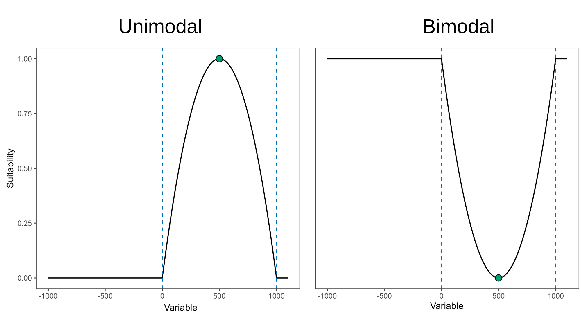
Figure 1. Representation of convex (left) and concave (right) response curves. Dashed lines indicate limits of environmental conditions for model training.
In our example, none of the maxnet selected models have concave responses, but the GLM selected had at least one concave response:
#Selected maxnet models
m_maxnet$selected_models[, c("ID", "Formulas", "Is_concave")]
#>      ID
#> 192 192
#> 219 219
#>                                                                                      Formulas
#> 192                        ~bio_1 + bio_7 + bio_15 + I(bio_1^2) + I(bio_7^2) + I(bio_15^2) -1
#> 219 ~bio_1 + bio_7 + bio_12 + bio_15 + I(bio_1^2) + I(bio_7^2) + I(bio_12^2) + I(bio_15^2) -1
#>     Is_concave
#> 192      FALSE
#> 219      FALSE

#Selected glm models
m_glm$selected_models[, c("ID", "Formulas", "Is_concave")]
#>    ID                                                        Formulas
#> 85 85 ~bio_1 + bio_7 + bio_12 + I(bio_1^2) + I(bio_7^2) + I(bio_12^2)
#>    Is_concave
#> 85       TRUE
This shows that a model with concave responses could be selected if
it has low omission rate and AIC values. To ensure that none of
the selected models have concave curves, you can set
remove_concave = TRUE within the calibration()
function. Let’s test it with the maxnet algorithm:
m_unimodal <- calibration(data = d_maxnet,
                          remove_concave = TRUE,  # Ensures concave models are not selected
                          error_considered = c(5, 10),
                          omission_rate = 10)
# Task 1/2: checking for concave responses in models:
#   |=====================================================================| 100%
#
# Task 2/2: fitting and evaluating models with no concave responses:
#   |=====================================================================| 100%
#
# Model selection step:
# Selecting best among 300 models.
# Calculating pROC...
#
# Filtering 300 models.
# Removing 0 model(s) because they failed to fit.
# Removing 39 model(s) with concave curves.
# 110 models were selected with omission rate below 10%.
# Selecting 2 final model(s) with delta AIC <2.
# Validating pROC of selected models...
#   |=====================================================================| 100%
# All selected models have significant pROC values.
Note that the process is now divided into two tasks:
Task 1: Only candidate models that include quadratic terms are fitted. For GLMs, all models with quadratic terms are tested. For maxnet models, the version of the models with quadratic terms with the highest regularization multiplier is tested. This is because if a maxnet model produces a concave response at a high regularization value, it will do the same at lower values.
Task 2: In this step, the function fits and evaluates two groups of models: (1) models without quadratic terms; and (2) models with quadratic terms, but only those with formulas that did not produce concave responses in Task 1.
Re-selecting models
The model selection procedure is conducted internally during the calibration process. However, it is possible to re-select models by considering other omission rates (since these were calculated during calibration), model complexity (delta AIC), and removing or not models with concave responses.
To optimize computational time, calibration() calculates
pROC values only for models pre-selected based on omission and
complexity considerations (default). Consequently, pROC values for
models that were not pre-selected are filled with NA.
# See first rows of the summary of calibration results (pROC values)
head(m_maxnet$calibration_results$Summary[, c("ID", "Mean_AUC_ratio_at_10.mean",
                                              "pval_pROC_at_10.mean")])
#>   ID Mean_AUC_ratio_at_10.mean pval_pROC_at_10.mean
#> 1  1                        NA                   NA
#> 2  2                        NA                   NA
#> 3  3                        NA                   NA
#> 4  4                        NA                   NA
#> 5  5                        NA                   NA
#> 6  6                        NA                   NA
# See pROC values of selected models
m_maxnet$selected_models[, c("ID", "Mean_AUC_ratio_at_10.mean",
                             "pval_pROC_at_10.mean")]
#>      ID Mean_AUC_ratio_at_10.mean pval_pROC_at_10.mean
#> 192 192                  1.497376                    0
#> 219 219                  1.502309                    0
When pROC is not calculated for all models during calibration, the
select_models() function requires to set
compute_proc = TRUE to obtain the necessary results for
selections with new criteria. Let’s re-select maxnet models applying an
omission rate of 5% instead 10%:
# Re-select maxnet models
new_m_maxnet <- select_models(calibration_results = m_maxnet,
                              compute_proc = TRUE,
                              omission_rate = 5)  # New omission rate
#> Selecting best among 300 models.
#> Calculating pROC...
#>
#> Filtering 300 models.
#> Removing 0 model(s) because they failed to fit.
#> 116 model(s) were selected with omission rate below 5%.
#> Selecting 2 final model(s) with delta AIC <2.
#> Validating pROC of selected models...
#>
#> All selected models have significant pROC values.

print(new_m_maxnet)
#> calibration_results object summary (maxnet)
#> =============================================================
#> Species: Myrcia hatschbachii
#> Number of candidate models: 300
#>   - Models removed because they failed to fit: 0
#>   - Models identified with concave curves: 39
#>   - Model with concave curves not removed
#>   - Models removed with non-significant values of pROC: 0
#>   - Models removed with omission error > 5%: 184
#>   - Models removed with delta AIC > 2: 114
#> Selected models: 2
#>   - Up to 5 printed here:
#>      ID                                                           Formulas
#> 159 159                        ~bio_1 + bio_7 + I(bio_1^2) + I(bio_7^2) -1
#> 189 189 ~bio_1 + bio_7 + bio_12 + I(bio_1^2) + I(bio_7^2) + I(bio_12^2) -1
#>     Features R_multiplier pval_pROC_at_5.mean Omission_rate_at_5.mean      dAIC
#> 159       lq          0.1                   0                  0.0192 0.8581936
#> 189       lq          0.1                   0                  0.0192 0.0000000
#>     Parameters
#> 159          4
#> 189          6
If a calibration_results object is provided,
select_models() will return a
calibration_results output with the selected models and
summary updated. Note that we now have different selected models with
the maxnet algorithm:
new_m_maxnet$selected_models[,c("ID", "Formulas", "R_multiplier",
                                "Omission_rate_at_5.mean",
                                "Mean_AUC_ratio_at_5.mean",
                                "AICc", "Is_concave")]
#>      ID                                                           Formulas
#> 159 159                        ~bio_1 + bio_7 + I(bio_1^2) + I(bio_7^2) -1
#> 189 189 ~bio_1 + bio_7 + bio_12 + I(bio_1^2) + I(bio_7^2) + I(bio_12^2) -1
#>     R_multiplier Omission_rate_at_5.mean Mean_AUC_ratio_at_5.mean     AICc
#> 159          0.1                  0.0192                 1.481338 622.7677
#> 189          0.1                  0.0192                 1.514759 621.9095
#>     Is_concave
#> 159      FALSE
#> 189      FALSE
You can also provide a data.frame containing the
evaluation metrics for each candidate model directly to
select_models(). This data.frame is available
in the output of the calibration() function under
object$calibration_results$Summary. In this case, the
function will return a list containing the selected models along with
summaries of the model selection process.
#Re-select models using data.frame
new_summary <- select_models(candidate_models = m_maxnet$calibration_results$Summary,
                             data = d_maxnet,  # Needed to compute pROC
                             compute_proc = TRUE,
                             omission_rate = 5)
#> Selecting best among 300 models.
#> Calculating pROC...
#>
#> Filtering 300 models.
#> Removing 0 model(s) because they failed to fit.
#> 116 model(s) were selected with omission rate below 5%.
#> Selecting 2 final model(s) with delta AIC <2.
#> Validating pROC of selected models...
#>
#> All selected models have significant pROC values.

#Get class of object
class(new_summary)
#> [1] "list"

#See selected models
new_summary$selected_models[, c("ID", "Formulas", "R_multiplier",
                                "Omission_rate_at_5.mean",
                                "Mean_AUC_ratio_at_5.mean",
                                "AICc", "Is_concave")]
#>      ID                                                           Formulas
#> 159 159                        ~bio_1 + bio_7 + I(bio_1^2) + I(bio_7^2) -1
#> 189 189 ~bio_1 + bio_7 + bio_12 + I(bio_1^2) + I(bio_7^2) + I(bio_12^2) -1
#>     R_multiplier Omission_rate_at_5.mean Mean_AUC_ratio_at_5.mean     AICc
#> 159          0.1                  0.0192                 1.479856 622.7677
#> 189          0.1                  0.0192                 1.511620 621.9095
#>     Is_concave
#> 159      FALSE
#> 189      FALSE
Training partition effects
After model calibration, selected models can be explored to understand the effect of leaving testing data out in every cross-validation process. This can help understand if leaving a testing partition out changes dramatically response curves compared to using other sets of data. These explorations can also be used to understand if the ability of models to predict testing records derives from extrapolation or not, and whether extrapolations are safe.
The function partition_response_curves() can be used to
perform the explorations mentioned above for each of the selected models
in the calibration_results object.
# ID of models that were selected
m_maxnet$selected_models$ID
#> [1] 192 219

# Response curves for model 192
partition_response_curves(calibration_results = m_maxnet, modelID = 192)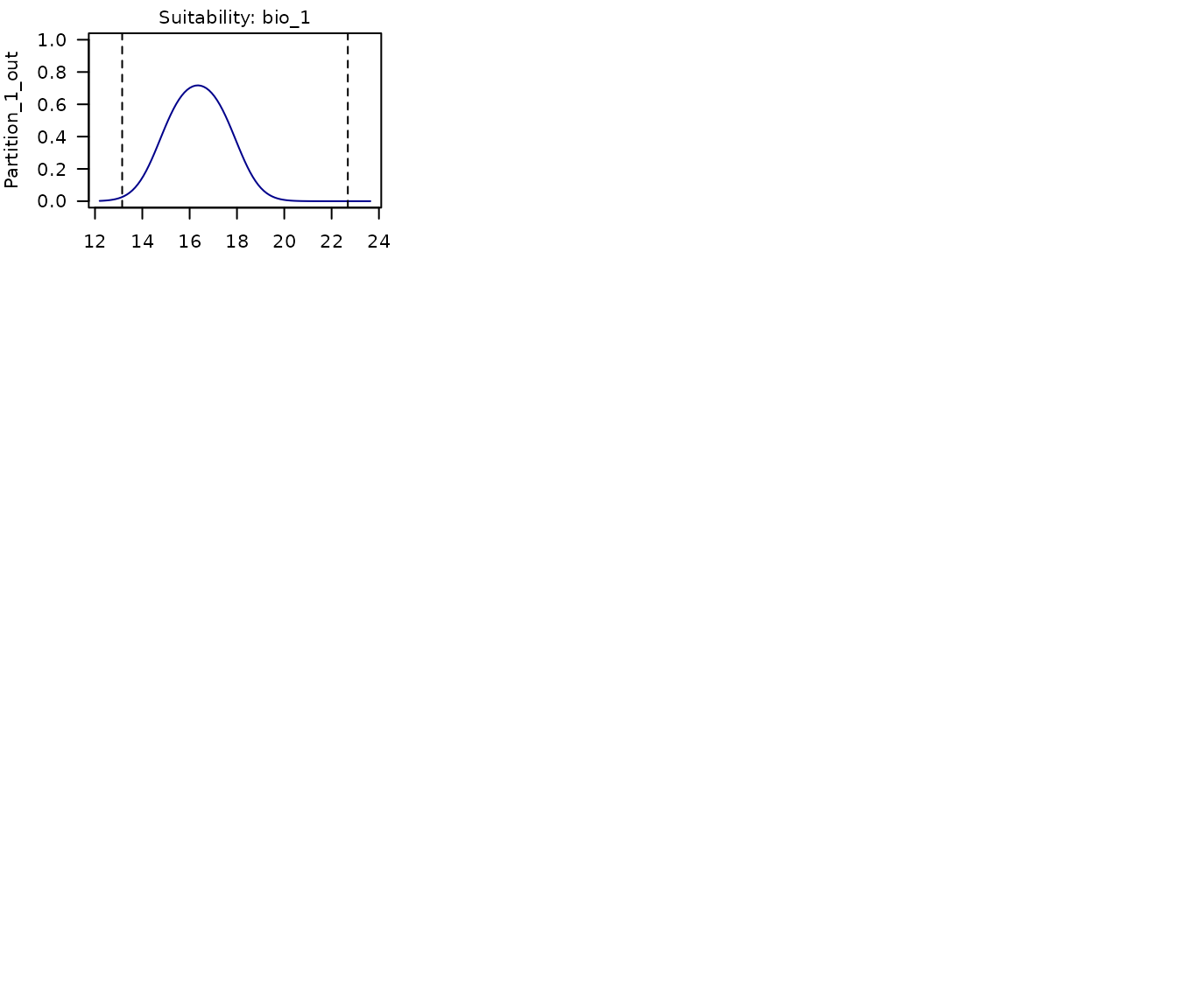
In the multi-panel plot produced above, we can see the response curves for each of the variables used in the model. Each panel shows:
- The response curve for the variable in a model fit with a portion of the data that leaves out the partition labeled in the y axis.
- Points of records used for testing, the ones corresponding to the partition left out.
- Dashed lines representing the limits of the environmental values in the data used to fit models.
The same can be done for each of the models selected. Below is a plot for the second model selected in this example.
# Response curves for model 219
partition_response_curves(calibration_results = m_maxnet, modelID = 219)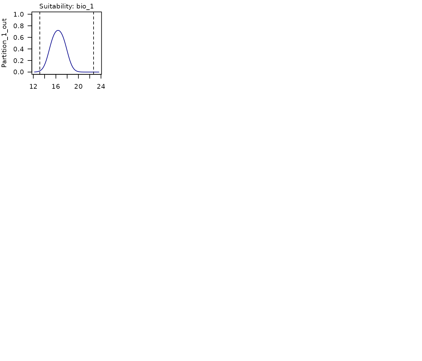
# Reset plotting parameters
par(original_par)
Saving a calibration_results object
After calibrating and selecting the best-performing models, we can
proceed to fit the final models (see the vignette for model exploration)
using the calibration_results object. As this object is
essentially a list, users can save it to a local directory using
saveRDS(). Saving the object facilitates loading it back
into your R session later using readRDS(). See an example
below: