5. Project Models to a Single Scenario • kuenm2

Summary

Description
Getting ready
Fitted models
Model predictions
- Predict to SpatRaster
- Predict to data.frame
Options for predictions
Binarize predictions
Saving Predictions
Detecting changes in predictions

Description

Once selected models have been fit and explored, projections to single or multiple scenarios can be performed. The predict_selected() function is designed for projections to single scenarios (i.e., a single set of new data). This vignette contains examples of how to use many of the options available for model predictions.

Getting ready

At this point it is assumed that kuenm2 is installed (if not, see the Main guide). Load kuenm2 and any other required packages, and define a working directory (if needed).

Note: functions from other packages (i.e., not from base R or kuenm2) used in this guide will be displayed as package::function().

# Load packages
library(kuenm2)
library(terra)

# Current directory
getwd()

# Define new directory
#setwd("YOUR/DIRECTORY")  # uncomment and modify if setting a new directory

# Saving original plotting parameters
original_par <- par(no.readonly = TRUE)

Fitted models

To predict using the selected models, a fitted_models object is required. For detailed information on model fitting, check the vignette Fit and Explore Selected Models. The fitted_models object generated in that vignette is included as an example dataset within the package. Let’s load it.

# Import fitted_model_maxnet
data("fitted_model_maxnet", package = "kuenm2")

# Print fitted models
fitted_model_maxnet
#> fitted_models object summary
#> ============================
#> Species: Myrcia hatschbachii 
#> Algortihm: maxnet 
#> Number of fitted models: 2 
#> Models fitted with 4 replicates

To compare the results, let’s import a fitted_models object generated using the GLM algorithm:

# Import fitted_model_glm
data("fitted_model_glm", package = "kuenm2")

# Print fitted models
fitted_model_glm
#> fitted_models object summary
#> ============================
#> Species: Myrcia hatschbachii 
#> Algortihm: glm 
#> Number of fitted models: 1 
#> Only full models fitted, no replicates

Model predictions

To predict selected models for a single scenario, you need a fitted_models object and the corresponding variables. These variables can be provided as either a SpatRaster or a data.frame. The names of the variables (or columns in the data.frame) must precisely match those used for model calibration or those used when running PCA (if do_pca = TRUE was set in the prepare_data() function; see Prepare Data for Model Calibration for more details).

Predict to SpatRaster

Let’s use the same raster variables that were used to prepare the data and calibrate the models. These are included as example data within the package:

# Import raster layers
var <- rast(system.file("extdata", "Current_variables.tif", package = "kuenm2"))

# Plot raster layers
terra::plot(var)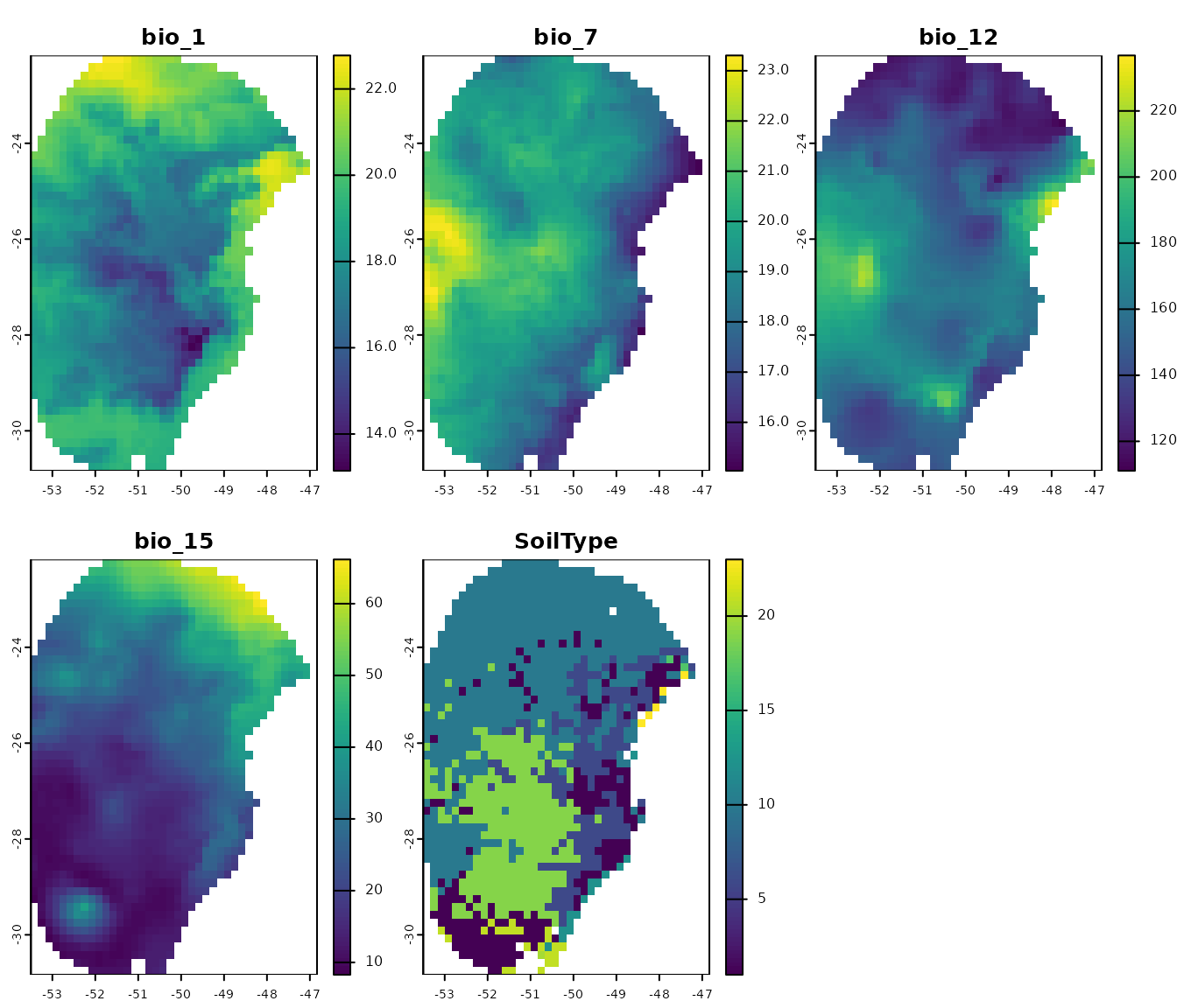

Let’s check which variables were used to calibrate our models. They are available in the calibration_data element of the object:

# Variables used to calibrate maxnet models
colnames(fitted_model_maxnet$calibration_data)
#> [1] "pr_bg"    "bio_1"    "bio_7"    "bio_12"   "bio_15"   "SoilType"

# Variables used to calibrate glms
colnames(fitted_model_glm$calibration_data)
#> [1] "pr_bg"    "bio_1"    "bio_7"    "bio_12"   "bio_15"   "SoilType"

The first column, “pr_bg”, indicates the presence (1) and background (0) records, while the other columns represent the environmental variables. In this case, the variables are bio_1, bio_7, bio_12, bio_15, and SoilType. All these variables are present in the SpatRaster (var) imported, so, we can predict our models to this raster. Let’s begin by predicting the maxnet model:

p_maxnet <- predict_selected(models = fitted_model_maxnet, new_variables = var,
                             progress_bar = FALSE)

By default, the function computes consensus metrics (mean, median, range, and standard deviation) for each model across its replicates (if they were produced), as well as a general consensus across all models (if multiple were selected). In this case, the output is a list containing SpatRasters for predictions, the consensus for each model, and the general consensus:

# See objects in the output of predict_selected
names(p_maxnet)
#> [1] "Model_192"         "Model_219"         "General_consensus"

Let’s plot the general consensus:

terra::plot(p_maxnet$General_consensus)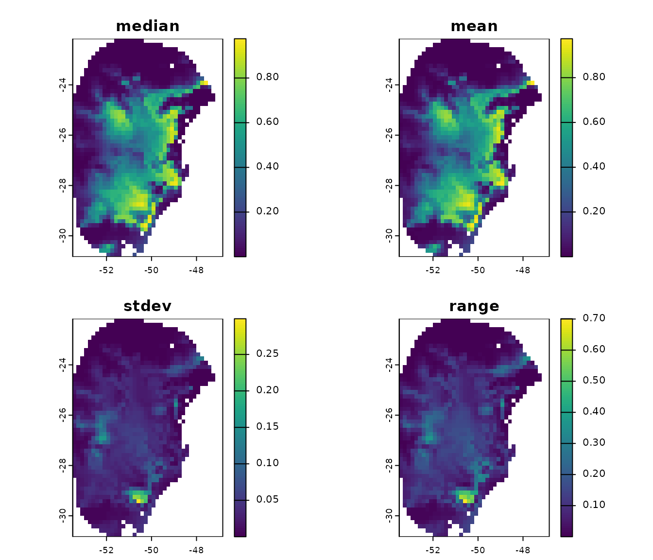

We can also plot the results for each replicate and the consensus for each model:

# Predictions for each replicate from model 192
terra::plot(p_maxnet$Model_192$Replicates)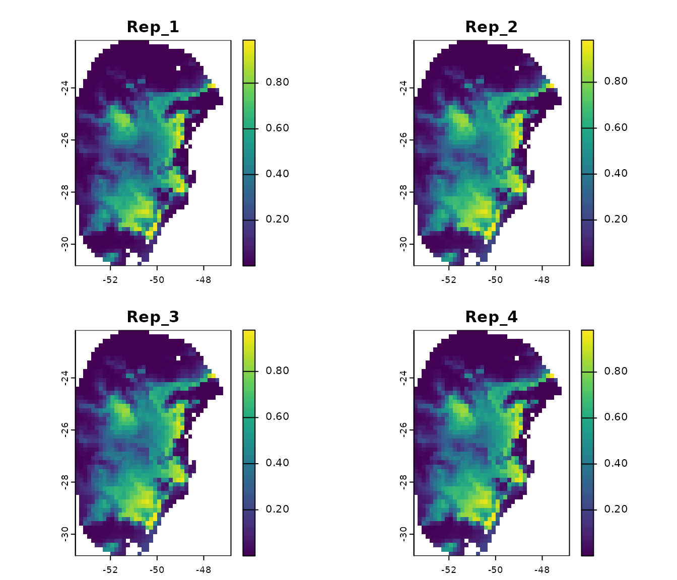


# Consensus across each replicate from model 192
terra::plot(p_maxnet$Model_192$Model_consensus)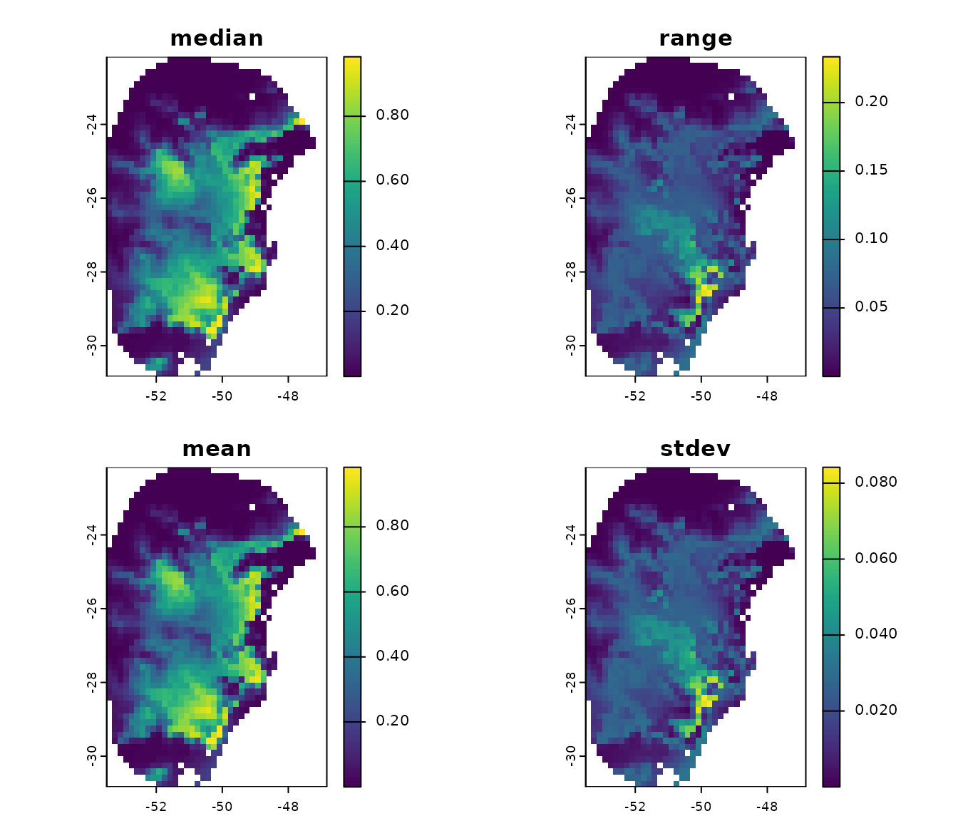

For comparison, let’s predict the GLM:

# Predict glm 
p_glm <- predict_selected(models = fitted_model_glm, 
                          new_variables = var,
                          progress_bar = FALSE)
# See selected models that were predicted
names(p_glm)
#> [1] "Model_85"          "General_consensus"

# Compare general consensus (mean) between maxnet and glm
par(mfrow = c(1, 2))  # Set grid to plot
terra::plot(p_maxnet$General_consensus$mean, main = "Maxnet")
terra::plot(p_glm$General_consensus, main = "GLM")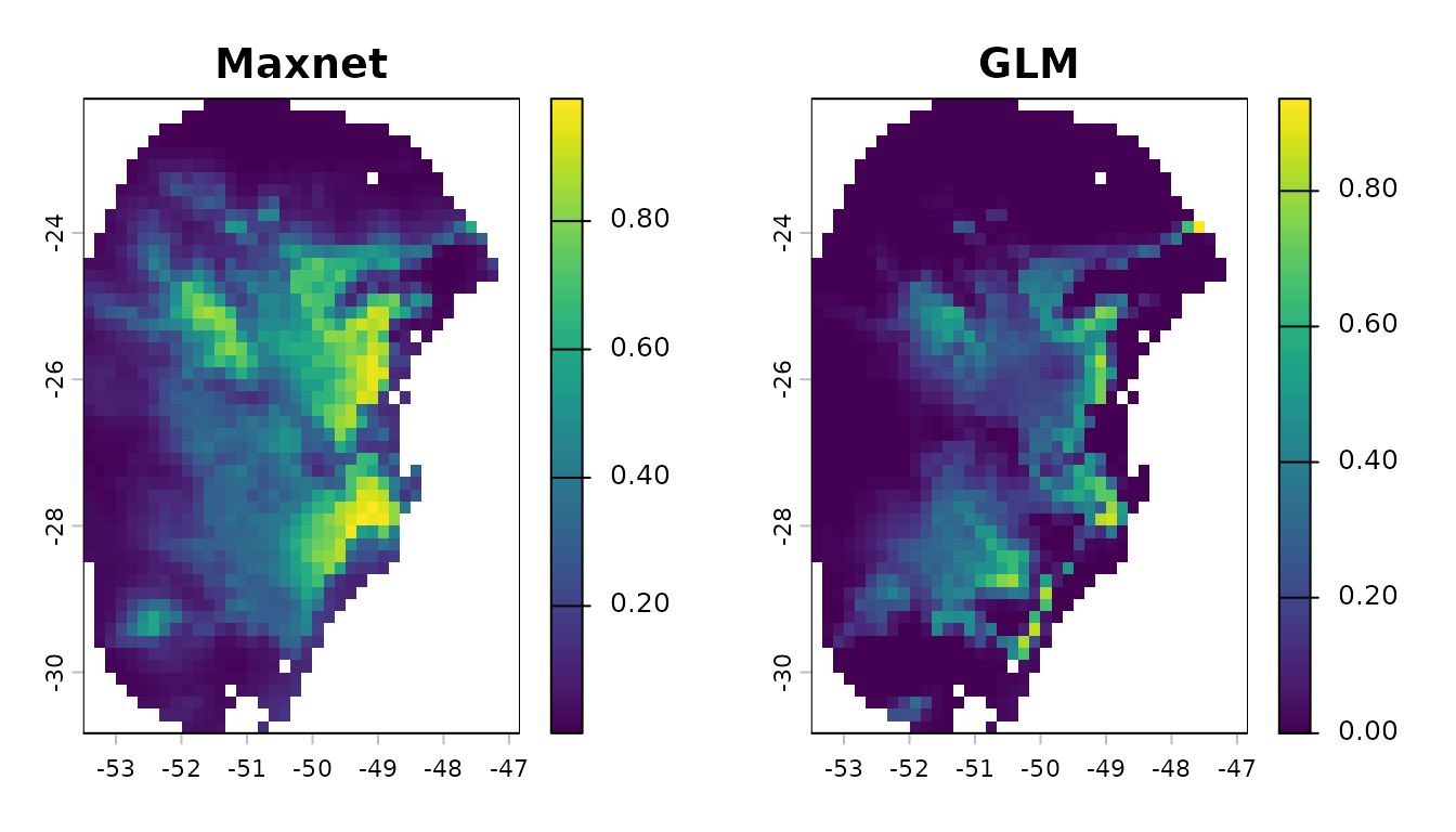

Predict to data.frame

Instead of a SpatRaster, we can also predict the models to a data.frame with the variable values. As an example, let’s convert the raster variables var to a data.frame:

var_df <- as.data.frame(var)
head(var_df)
#>       bio_1    bio_7 bio_12   bio_15 SoilType
#> 11 22.77717 18.12400   1180 48.03594       NA
#> 12 22.76711 17.74400   1191 49.31194       10
#> 13 22.68580 17.46575   1206 51.51922       10
#> 14 22.50121 17.84525   1228 53.90265       10
#> 15 22.07609 18.14125   1254 54.10397       10
#> 16 21.88485 18.80800   1276 54.07279       10

Note that each column stores the values for each variable. Let’s predict our Maxnet models to this data.frame:

p_df <- predict_selected(models = fitted_model_maxnet, 
                         new_variables = var_df,  # Now, a data.frame
                         progress_bar = FALSE)

Now, instead of SpatRaster objects, the function returns data.frame objects with the predictions:

# Results by replicate of the model 192
head(p_df$Model_192$Replicates)
#>   Replicate_1  Replicate_2  Replicate_3  Replicate_4
#> 1 0.006521501 0.0006209852 0.0005883615 9.831561e-05
#> 2 0.006446437 0.0005356316 0.0005713501 9.009486e-05
#> 3 0.006233583 0.0003396879 0.0004975279 6.967025e-05
#> 4 0.005797668 0.0001458500 0.0003605775 4.303576e-05
#> 5 0.008513515 0.0002034105 0.0006532983 8.529550e-05
#> 6 0.009240381 0.0001753492 0.0006784553 9.035171e-05

# Consensus across replicates of the model 192
head(p_df$Model_192$Model_consensus)
#>         median       range        mean       stdev
#> 1 0.0006046734 0.006423186 0.001957291 0.003052184
#> 2 0.0005534909 0.006356342 0.001910878 0.003031621
#> 3 0.0004186079 0.006163912 0.001785117 0.002970901
#> 4 0.0002532137 0.005754632 0.001586783 0.002810372
#> 5 0.0004283544 0.008428219 0.002363880 0.004107054
#> 6 0.0004269022 0.009150029 0.002546134 0.004470371

# General consensus across all models
head(p_df$General_consensus)
#>         median       range        mean       stdev
#> 1 0.0006049792 0.006423186 0.001882943 0.002691096
#> 2 0.0005534909 0.006356342 0.001847258 0.002690840
#> 3 0.0004186079 0.006163912 0.001737935 0.002664381
#> 4 0.0002532730 0.005757458 0.001562733 0.002558575
#> 5 0.0004283544 0.008435158 0.002337815 0.003756587
#> 6 0.0004274250 0.009165160 0.002539356 0.004130584

Options for predictions

Output type

Maxnet models produce four different types of output for their predictions: raw, cumulative, logistic, and cloglog. These are described in Merow et al. 2013 and Phillips et al. 2017.

All four output types are monotonically related; thus, rank-based metrics for model fit (e.g., omission rate and partial ROC) will be identical. However, the output types have different scaling, which leads to distinct interpretations and visually different prediction maps.

Raw (or exponential) output is interpreted as a Relative Occurrence Rate (ROR). The ROR sums to 1 when predicted to the data used to train the model.
Cumulative output assigns to a location the sum of all raw values less than or equal to the raw value for that location, and then rescales this to range between 0 and 100. Cumulative output can be interpreted in terms of an omission rate because thresholding at a value of c to predict a suitable/unsuitable cell will omit approximately c% of presences.
Cloglog output (Default) transforms the raw values into a scale of relative suitability ranging between 0 and 1, using a logistic transformation based on a user-specified parameter ‘ $\tau$ ’, which represents the probability of presence at ‘average’ presence locations. In this context, the tau value defaults to $\tau \approx 0.632$ .
Logistic output is similar to Cloglog, but it assumes that $\tau = 0.5$ .

Let’s examine the differences between these four output types for Maxnet models:

p_cloglog <- predict_selected(models = fitted_model_maxnet, new_variables = var, 
                              type = "cloglog", progress_bar = FALSE)
p_logistic <- predict_selected(models = fitted_model_maxnet, new_variables = var, 
                              type = "logistic", progress_bar = FALSE)
p_cumulative <- predict_selected(models = fitted_model_maxnet, new_variables = var, 
                                 type = "cumulative", progress_bar = FALSE)
p_raw <- predict_selected(models = fitted_model_maxnet, new_variables = var, 
                          type = "raw", progress_bar = FALSE)

# Plot the differences
par(mfrow = c(2, 2))
terra::plot(p_cloglog$General_consensus$mean, main = "Cloglog (Default)",
            zlim = c(0, 1))
terra::plot(p_logistic$General_consensus$mean, main = "Logistic", 
            zlim = c(0, 1))
terra::plot(p_cumulative$General_consensus$mean, main = "Cumulative",
            zlim = c(0, 1))
terra::plot(p_raw$General_consensus$mean, main = "Raw", zlim = c(0, 1))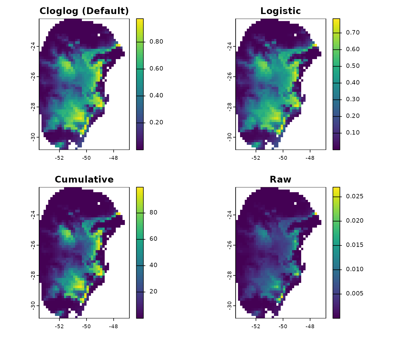

Clamping variables

By default, predictions are performed with free extrapolation (extrapolation_type = "E"). This can be problematic when the peak of suitability occurs at the extremes of a variable’s range. For example, let’s examine the response curve of the Maxnet model for bio_7 (Temperature Annual Range):

response_curve(models = fitted_model_maxnet, variable = "bio_7", 
               extrapolation_factor = 1)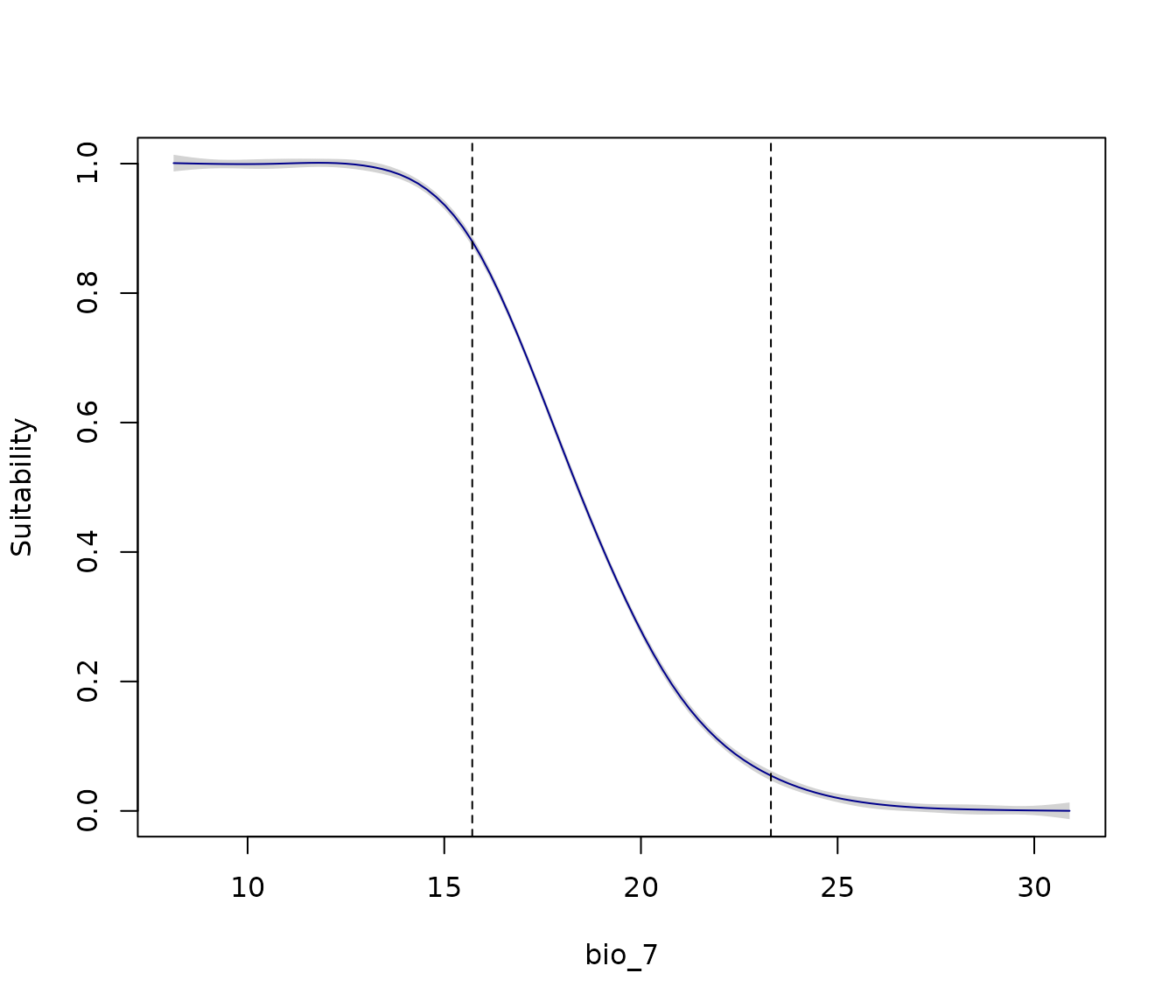

Note that higher suitability occurs at low values of the temperature range. However, the lower limit of the calibration data used to fit the models (dashed line) is at 15.7ºC. The premise that suitability will increase and stabilize at lower values of bio_7 is an extrapolation of the model (the area to the left of the dashed line). It’s possible that suitability decreases at extremely low values, but training data is insufficient for the model to predict this.

One way to address this is by clamping the variables. This means that all prediction values outside the training range (both below the lower value and above the upper value) are set to the prediction values found at the limits of the range. For example, in the calibration data for the Maxnet models, the lower and upper limits for bio_7 are 15.7ºC and 23.3ºC, respectively:

range(fitted_model_maxnet$calibration_data$bio_7)
#> [1] 15.71120 23.30475

To observe the effect of clamping this variable, let’s create a hypothetical scenario where bio_7 has very low values:

# From bio_7, reduce values
new_bio7 <- var$bio_7 - 3

# Create new scenario
new_var <- var

# Replace bio_7 with new_bio7 in this scenario
new_var$bio_7 <- new_bio7

# Plot the differences
par(mfrow = c(1, 2))
terra::plot(var$bio_7, main = "Original bio_7", range = c(5, 25))
terra::plot(new_var$bio_7, main = "New bio_7", range = c(5, 25))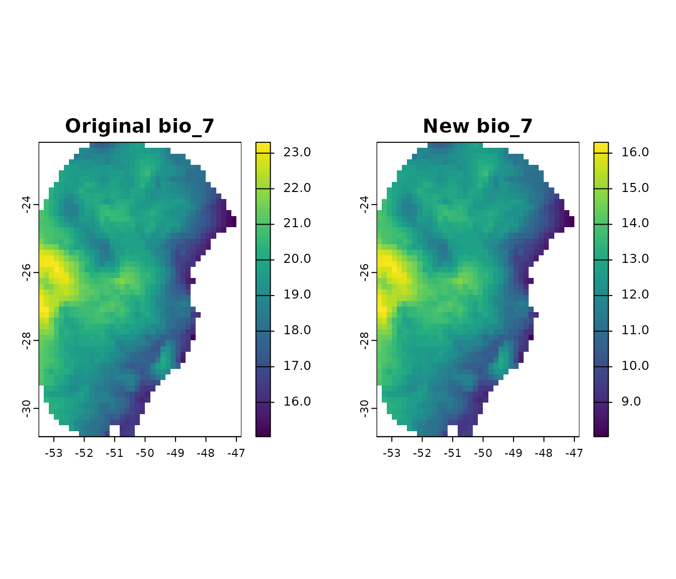

Let’s predict the Maxnet models for this new scenario with both free extrapolation (extrapolation_type = "E") and with clamped variables (extrapolation_type = "EC"):

# Predict to hypothetical scenario with free extrapolation
p_free_extrapolation <- predict_selected(models = fitted_model_maxnet, 
                                         new_variables = new_var,  # New scenario
                                         consensus = "mean",
                                         extrapolation_type = "E",  # Free extrapolation (Default)
                                         progress_bar = FALSE)

# Predict to hypothetical scenario with clamping
p_clamping <- predict_selected(models = fitted_model_maxnet, 
                               new_variables = new_var,  # New scenario
                               consensus = "mean",
                               extrapolation_type = "EC",  # Extrapolation with clamping
                               progress_bar = FALSE)

# Get and see differences
p_difference <- p_free_extrapolation$General_consensus$mean - p_clamping$General_consensus$mean

# Plot the differences
par(mfrow = c(2, 2))
terra::plot(p_free_extrapolation$General_consensus$mean, 
            main = "Free extrapolation", zlim = c(0, 1))
terra::plot(p_clamping$General_consensus$mean, main = "Clamping",
             zlim = c(0, 1))
terra::plot(p_difference, main = "Difference")
terra::plot(new_bio7, main = "Hypothetical bio_7", type = "interval")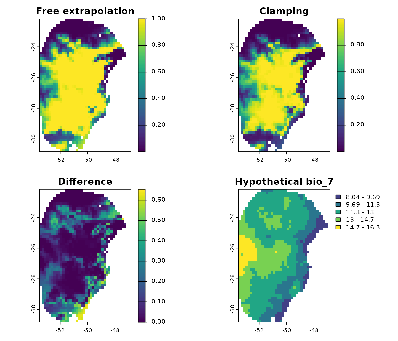

Note that when we clamp the variables, regions with extremely low values of (the hypothetical) bio_7 exhibit lower predicted suitability values compared to when free extrapolation is allowed.

By default, when extrapolation_type = "EC" is set, all variables are clamped. You can specify which variables to clamp using the var_to_restrict argument.

No extrapolation

A more rigorous approach is to predict with no extrapolation. Here regions outside the limits of the training data are assigned a suitability value of 0. Let’s proceed to observe the differences:

# Predict to hypothetical scenario with no extrapolation
p_no_extrapolation <- predict_selected(models = fitted_model_maxnet, 
                                       new_variables = new_var,  # New scenario
                                       consensus = "mean",
                                       extrapolation_type = "NE",  # No extrapolation
                                       progress_bar = FALSE)
# Plot the differences
par(mfrow = c(2, 2))
terra::plot(p_free_extrapolation$General_consensus$mean, main = "Free extrapolation",
            zlim = c(0, 1))
terra::plot(p_clamping$General_consensus$mean, main = "Clamping",
            zlim = c(0, 1))
terra::plot(p_no_extrapolation$General_consensus$mean, main = "No extrapolation",
            zlim = c(0, 1))
terra::plot(new_bio7, main = "Hypothetical bio_7", type = "interval")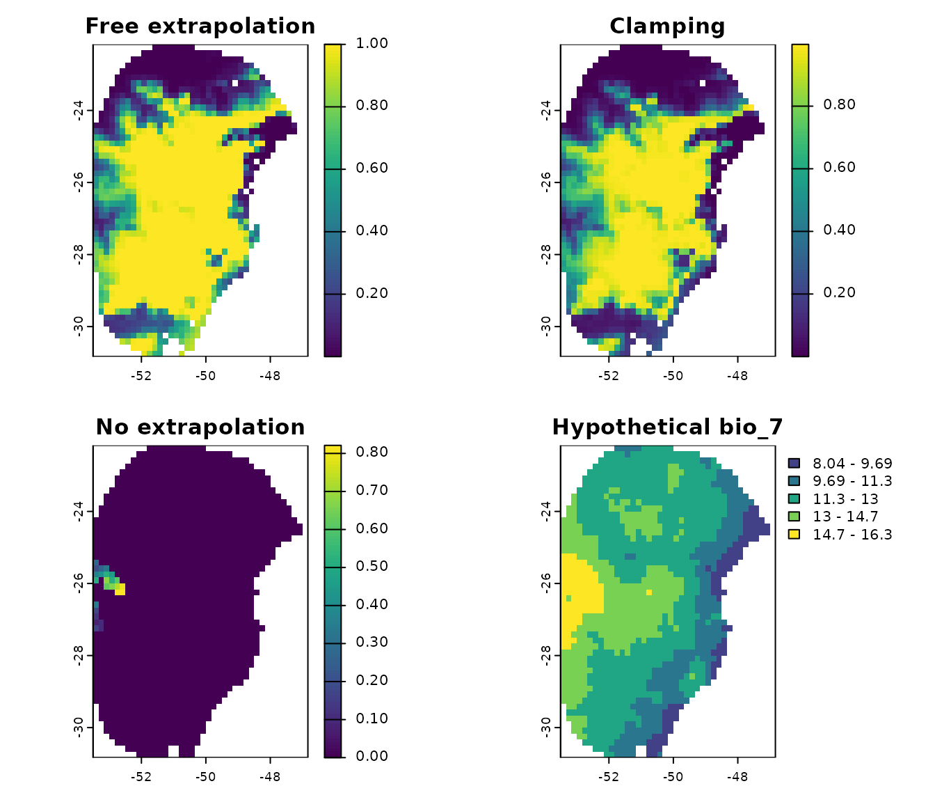

In this example, a large portion of the predicted area shows zero suitability. This is because, in this hypothetical scenario, much of the region has bio_7 values lower than those in the training data, which has a minimum of 15ºC. Suitability values greater than zero are only in areas where bio_7 falls within the training range.

By default, when extrapolation_type = "NE" is set, all variables are considered for this process. You can specify a subset of variables to be considered for extrapolation using the var_to_restrict argument.

Binarize predictions

The fitted_models object stores the thresholds that can be used to classify model predictions into suitable and unsuitable areas. These thresholds correspond to the omission error rate used during model selection (e.g., 5% or 10%).

You can access the omission error rate used to calculate the thresholds directly from the object:

# Get omission error used to select models and calculate the thesholds
## For maxnet model
fitted_model_maxnet$omission_rate
#> [1] 10

## For glm
fitted_model_glm$omission_rate
#> [1] 10

In both models, a 10% omission error rate was used to calculate the thresholds. This means that when predictions are binarized, approximately 10% of the presence records used to train models will fall into areas classified as unsuitable.

The thresholds are summarized in two ways: the mean and median across replicates for each model, and the consensus mean and median across all selected models (when more than one model is selected). Let’s check the thresholds for the general consensus:

# For maxnet
fitted_model_maxnet$thresholds$consensus
#> $mean
#> [1] 0.3095083
#> 
#> $median
#> [1] 0.259534

# For glm
fitted_model_glm$thresholds$consensus
#> $mean
#> [1] 0.1204713
#> 
#> $median
#> [1] 0.1204713

Let’s use these threshold values to binarize models predictions:

# Get the threshold values for models (general consensus)
thr_mean_maxnet <- fitted_model_maxnet$thresholds$consensus$mean  # Maxnet
thr_mean_glm <- fitted_model_glm$thresholds$consensus$mean  # glm

# Binarize models
mean_maxnet_bin <- (p_maxnet$General_consensus$mean >= thr_mean_maxnet) * 1
mean_glm_bin <- (p_glm$General_consensus >= thr_mean_glm) * 1

# Compare results
par(mfrow = c(1, 2))  # Set grid to plot
terra::plot(mean_maxnet_bin, main = "Maxnet")
terra::plot(mean_glm_bin, main = "GLM")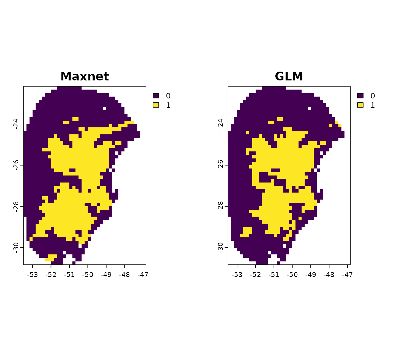

# Reset plotting parameters
par(original_par)

Saving predictions

We can save the predictions to the disk by setting write_files = TRUE. When this option is enabled, you must provide a directory path in the out_dir argument.

If new_variables is a SpatRaster, the function will save files as GeoTIFF (.tif) files. If new_variables is a data.frame, the function will save the output files as Comma Separated Value (.csv) files.

p_save <- predict_selected(models = fitted_model_maxnet, 
                           new_variables = var, 
                           write_files = TRUE,  # To save to the disk
                           write_replicates = TRUE,  # To save predictions for each replicate
                           out_dir = tempdir(),  # Directory to save the results (temporary directory)
                           progress_bar = FALSE)

Alternatively, we can use writeRaster() to save specific output predictions manually. For example, to save only the mean layer from the general consensus results:

terra::writeRaster(p_maxnet$General_consensus$mean, 
                   filename = file.path(tempdir(), "Mean_consensus.tif"))

Detecting changes in predictions

To compare predictions between two single scenarios representing different time periods (e.g., present vs. future or present vs. past), the function prediction_changes() can be used. This function helps to identify loss (contraction), gain (expansion), and stability (no change) of suitable areas.

As an example, we will project the fitted model to a single GCM representing future climatic conditions:

# Read layers representing future conditions
future_var <- terra::rast(system.file("extdata",
                                      "wc2.1_10m_bioc_ACCESS-CM2_ssp585_2081-2100.tif",
                                      package = "kuenm2"))

# Plot future layers
terra::plot(future_var)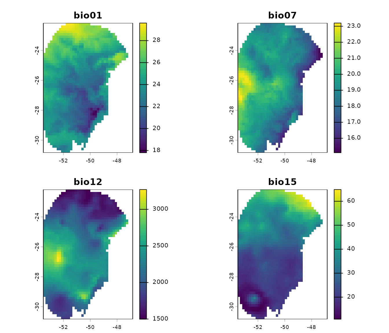

Next, we need to rename the variables so that they match the variable names used when fitting the models. After that, we will also append the static soil variable to the set of future variables.

# renaming layers to match names of variables used to fit the model
names(future_var) <- sub("bio0", "bio", names(future_var))
names(future_var) <- sub("bio", "bio_", names(future_var))
names(var)
#> [1] "bio_1"    "bio_7"    "bio_12"   "bio_15"   "SoilType"
names(future_var)
#> [1] "bio_1"  "bio_7"  "bio_12" "bio_15"

# Adding soil layer to future variable set
future_var <- c(future_var, var$SoilType)

Now we can generate predictions under future environmental conditions:

# Predict
p_future <- predict_selected(models = fitted_model_maxnet,
                             new_variables = future_var, 
                             progress_bar = FALSE)

# Plot consensus (mean)
terra::plot(c(p_maxnet$General_consensus$mean,
              p_future$General_consensus$mean),
            main = c("Present", "Future (SSP 585, 2081-2100)"))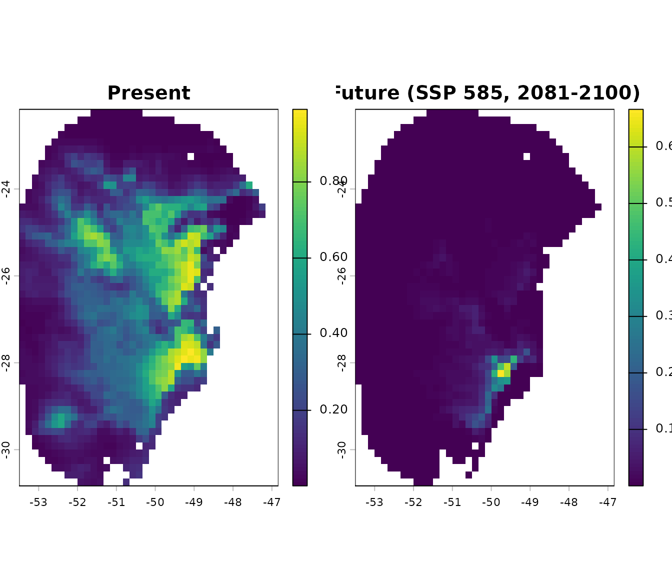

To identify how suitable areas change between scenarios, we can use prediction_changes(). This function computes binary layers from the predictions using the threshold stored in the fitted models, compares current and future predictions, and then classifies each cell as gain, loss, or stable.

# Compute changes between scenarios
p_changes <- prediction_changes(current_predictions = p_maxnet$General_consensus$mean,
                                new_predictions = p_future$General_consensus$mean,
                                fitted_models = fitted_model_maxnet,
                                predicted_to = "future")

# Plot result
terra::plot(p_changes)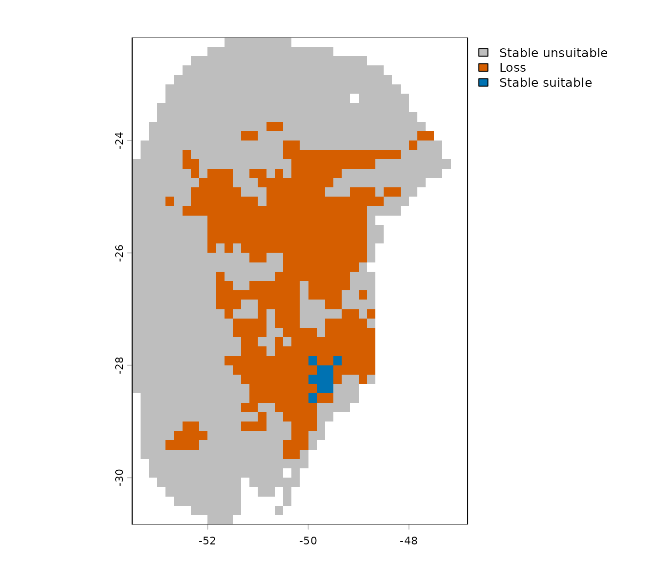

In this example, we are comparing current and future predictions, so we set predicted_to = "future". If a comparison with past predictions is needed, this argument should be set accordingly to ensure that categories of change or stability are assigned correctly.

The prediction_changes() function is designed to compute changes between single scenarios, meaning that the new scenario is represented by one set of layers. If projections include multiple GCMs, the function projection_changes() should be used instead. For more details on projecting models and detecting changes with summaries across multiple scenarios, see the vignette 6. Project Models to Multiple Scenarios.