Set Colors for Change Maps

This functions sets the color tables associated with the SpatRaster object resulting from projection_changes(). Color tables are used to associate specific colors with raster values when using plot(). This function defines custom colors for areas of gain, loss, and stability across scenarios.

Usage

colors_for_changes(
  changes_projections,
  gain_color = "#009E73",
  loss_color = "#D55E00",
  stable_suitable = "#0072B2",
  stable_unsuitable = "grey",
  max_alpha = 1,
  min_alpha = 0.25
)

Arguments

changes_projections

an object of class changes_projections, generated by projection_changes() or imported using import_projections(), containing the $Summary_changes element.

gain_color

(character) color used to define the pallete for representing gains. Default is "#009E73" (teal green).

loss_color

(character) color used to define the pallete for representing losses. Default is "#D55E00" (orange-red).

stable_suitable

(character) color used for representing areas that remain suitable across all scenarios. Default is "#0072B2" (oxford blue).

stable_unsuitable

(character) color used for representing areas that remain unsuitable across all scenarios. Default is "grey".

max_alpha

(numeric) opacity value (from 0 to 1) for areas where all GCMs agree on the change (gain, loss, or stability). Default is 1.

min_alpha

(numeric) opacity value (from 0 to 1) for areas where only one GCM predicts a given change. Default is 0.25

Value

An object of class changes_projections with the same structure and SpatRasters as the input changes_projections, but with color tables embedded in the SpatRasters. These colors are used automatically when visualizing the data with plot().

Examples

# Step 1: Organize variables for current projection
## Import current variables (used to fit models)
var <- terra::rast(system.file("extdata", "Current_variables.tif",
                               package = "kuenm2"))

## Create a folder in a temporary directory to copy the variables
out_dir_current <- file.path(tempdir(), "Current_raw_color_example")
dir.create(out_dir_current, recursive = TRUE)

## Save current variables in temporary directory
terra::writeRaster(var, file.path(out_dir_current, "Variables.tif"))


# Step 2: Organize future climate variables (example with WorldClim)
## Directory containing the downloaded future climate variables (example)
in_dir <- system.file("extdata", package = "kuenm2")

## Create a folder in a temporary directory to copy the future variables
out_dir_future <- file.path(tempdir(), "Future_raw_color_example")

## Organize and rename the future climate data (structured by year and GCM)
### 'SoilType' will be appended as a static variable in each scenario
organize_future_worldclim(input_dir = in_dir, output_dir = out_dir_future,
                          name_format = "bio_",
                          fixed_variables = var$SoilType)
#> 
  |                                                                            
  |                                                                      |   0%
  |                                                                            
  |=========                                                             |  12%
  |                                                                            
  |==================                                                    |  25%
  |                                                                            
  |==========================                                            |  38%
  |                                                                            
  |===================================                                   |  50%
  |                                                                            
  |============================================                          |  62%
  |                                                                            
  |====================================================                  |  75%
  |                                                                            
  |=============================================================         |  88%
  |                                                                            
  |======================================================================| 100%
#> 
#> Variables successfully organized in directory:
#> /tmp/Rtmphkhpn9/Future_raw_color_example

# Step 3: Prepare data to run multiple projections
## An example with maxnet models
## Import example of fitted_models (output of fit_selected())
data(fitted_model_maxnet, package = "kuenm2")

## Prepare projection data using fitted models to check variables
pr <- prepare_projection(models = fitted_model_maxnet,
                         present_dir = out_dir_current,
                         future_dir = out_dir_future,
                         future_period = c("2081-2100"),
                         future_pscen = c("ssp126", "ssp585"),
                         future_gcm = c("ACCESS-CM2", "MIROC6"),
                         raster_pattern = ".tif*")

# Step 4: Run multiple model projections
## A folder to save projection results
out_dir <- file.path(tempdir(), "Projection_results/maxnet_color_example")
dir.create(out_dir, recursive = TRUE)

## Project selected models to multiple scenarios
p <- project_selected(models = fitted_model_maxnet, projection_data = pr,
                      out_dir = out_dir)
#> 
  |                                                                            
  |                                                                      |   0%
  |                                                                            
  |==============                                                        |  20%
  |                                                                            
  |============================                                          |  40%
  |                                                                            
  |==========================================                            |  60%
  |                                                                            
  |========================================================              |  80%
  |                                                                            
  |======================================================================| 100%

# Step 5: Identify areas of change in projections
## Contraction, expansion and stability
changes <- projection_changes(model_projections = p, by_gcm = TRUE,
                              by_change = TRUE, write_results = FALSE,
                              return_raster = TRUE)

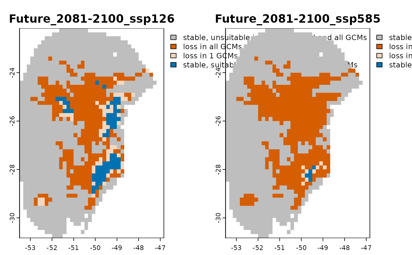
#Step 6: Set Colors for Change Maps
changes_with_colors <- colors_for_changes(changes_projections = changes)
terra::plot(changes_with_colors$Summary_changes)