Compute changes of suitable areas in other scenarios (single scenario / GCM)

Usage

prediction_changes(current_predictions, new_predictions,
                   predicted_to = "future", fitted_models = NULL,
                   consensus = "mean", user_threshold = NULL,
                   force_resample = FALSE, gain_color = "#009E73",
                   loss_color = "#D55E00", stable_suitable = "#0072B2",
                   stable_unsuitable = "grey", write_results = FALSE,
                   output_dir = NULL, overwrite = FALSE,
                   write_bin_models = FALSE)

Arguments

current_predictions: (SpatRaster) A SpatRaster object returned by predict_selected() with suitability predicted under current conditions.
new_predictions: (SpatRaster) A SpatRaster object returned by predict_selected() with suitability predicted under new conditions (past or future). This SpatRaster must have the same resolution and extent as current_predictions.
predicted_to: (character) a string specifying whether new_predictions represent "past" or "future" conditions. Default is "future".
fitted_models: an object of class fitted_models returned by fit_selected()
consensus: (character) the consensus metric stored in fitted_models used to binarize models. Available options are "mean", "median", "range", and "stdev" (standard deviation). Default is "mean".
user_threshold: (numeric) an optional threshold for binarizing predictions. Default is NULL, meaning the function will apply the thresholds stored in model_projections, which were calculated earlier using the omission rate from calibration().
force_resample: (logical) whether to force rasters to have the same extent and resolution. Default is TRUE.
gain_color: (character) color used to represent gains. Default is "#009E73" (teal green).
loss_color: (character) color used to represent losses. Default is "#D55E00" (orange-red).
stable_suitable: (character) color used for representing areas that remain suitable across scenarios. Default is "#0072B2" (oxford blue).
stable_unsuitable: (character) color used for representing areas that remain unsuitable across scenarios. Default is "grey".
write_results: (logical) whether to save the results to disk. Default is FALSE.
output_dir: (character) directory path where results will be saved. Only relevant if write_results = TRUE.
overwrite: (logical) whether to overwrite SpatRasters if they already exist. Only applicable if write_results = TRUE. Default is FALSE.
write_bin_models: (logical) whether to write the binarized models for each scenario to the disk. Only applicable if write_results = TRUE. Default is FALSE.

Value

A SpatRaster showing the areas of gain, loss and stability.

Details

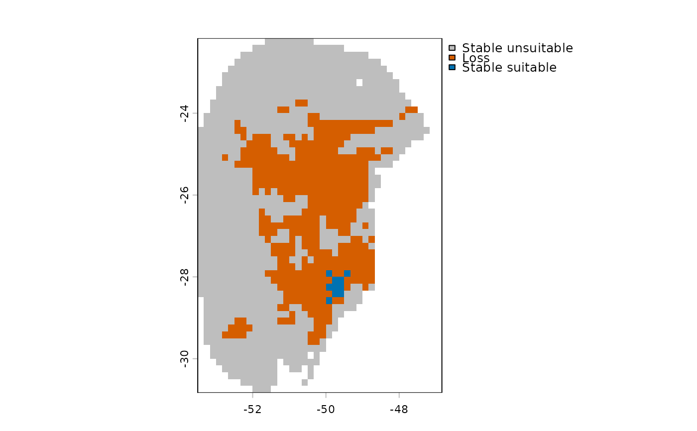
When projecting a niche model to different temporal scenarios (past or future), species’ areas can be classified into three categories relative to the current baseline: gain, loss and stability. The interpretation of these categories depends on the temporal direction of the projection. When projecting to future scenarios:

Gain: Areas that are currently unsuitable become suitable in the future.
Loss: Areas that are currently suitable become unsuitable in the future.
Stability: Areas that retain their current classification in the future, whether suitable or unsuitable.

When projecting to past scenarios:

Gain: Areas that were unsuitable in the past are now suitable in the present.
Loss: Areas that were suitable in the past are now unsuitable in the present.
Stability: Areas that retain their past classification in the present, whether suitable or unsuitable.

Examples

# Import an example of fitted models (output of fit_selected())
data("fitted_model_maxnet", package = "kuenm2")


# Import current variables for prediction
present_var <- terra::rast(system.file("extdata", "Current_variables.tif",
                                       package = "kuenm2"))


# Import variables for a single future scenario for prediction
future_var <- terra::rast(system.file("extdata",
                                      "wc2.1_10m_bioc_ACCESS-CM2_ssp585_2081-2100.tif",
                                      package = "kuenm2"))

# Rename variables to match the variable names used in the fitted models
names(future_var) <- sub("bio0", "bio", names(future_var))
names(future_var) <- sub("bio", "bio_", names(future_var))

# Append the static soil variable to the future variables
future_var <- c(future_var, present_var$SoilType)

# Predict under present and future conditions
p_present <- predict_selected(models = fitted_model_maxnet,
                              new_variables = present_var)
#> 
  |                                                                            
  |                                                                      |   0%
  |                                                                            
  |===================================                                   |  50%
  |                                                                            
  |======================================================================| 100%
p_future <- predict_selected(models = fitted_model_maxnet,
                             new_variables = future_var)
#> 
  |                                                                            
  |                                                                      |   0%
  |                                                                            
  |===================================                                   |  50%
  |                                                                            
  |======================================================================| 100%


# Compute changes between scenarios
p_changes <- prediction_changes(current_predictions = p_present$General_consensus$mean,
                                new_predictions = p_future$General_consensus$mean,
                                fitted_models = fitted_model_maxnet,
                                predicted_to = "future")
# Plot result
terra::plot(p_changes)