Occurrene Data Cleaning
basic_bata_cleaning.RmdDescription
As any modeling technique, ecological niche modeling depends on the quality of the input data, particularly species occurrence records. Cleaning these data is a critical step to minimize biases, reduce errors, and ensure meaningful model outcomes. This vignette introduces tools available in the kuenm2 package to facilitate the cleaning of occurrence data prior to modeling. It guides users through loading and inspecting data, applying cleaning functions, and saving cleaned datasets, all within a reproducible R workflow.
We want to highlight that additional data cleaning and filtering steps (e.g., spatial thinning) may be necessary depending on the type of model or modeling approach the user intends to adopt. The tools presented here are designed to assist with the most basic steps of preparing data for modeling.
Getting ready
If kuenm2 has not been installed yet, please do so. See the Main guide for installation instructions.
Load kuenm2 and any other required packages, and define a working directory (if needed). In general, setting a working directory in R is considered good practice, as it provides better control over where files are read from or saved to. If users are not working within an R project, we recommend setting a working directory, since at least one file will be saved at later stages of this guide.
# Load packages
library(kuenm2)
library(terra)

# Current directory
getwd()

# Define new directory
#setwd("YOUR/DIRECTORY")  # uncomment this line if setting a new directory
Cleaning data
Import data
We will use occurrence records provided within the
kuenm2 package. Most example data sets in the package
were derived from Trindade
& Marques (2024). The occ_data_noclean object
contains 51 valid occurrences of Myrcia hatschbachii (a tree
endemic to Southern Brazil) and a group of erroneous records to
demonstrate cleaning steps.
# Import occurrences
data(occ_data_noclean, package = "kuenm2")

# Check data structure
str(occ_data_noclean)
#> 'data.frame':    64 obs. of  3 variables:
#>  $ species: chr  "Myrcia hatschbachii" "Myrcia hatschbachii" "Myrcia hatschbachii" "Myrcia hatschbachii" ...
#>  $ x      : num  -51.3 -50.6 -49.3 -49.8 -50.2 ...
#>  $ y      : num  -29 -27.6 -27.8 -26.9 -28.2 ...
A raster layer from a group of layers include in the package will also be used in this example. This is a bioclimatic variable from WorldClim 2.1 at 10 arc-minute resolution. This layer has been masked using a polygon generated by drawing a minimum convex polygon around the records with a 300 km buffer.
# Import raster layers
var <- rast(system.file("extdata", "Current_variables.tif", package = "kuenm2"))

# Keep only one layer
var <- var$bio_1

# Check variable
plot(var)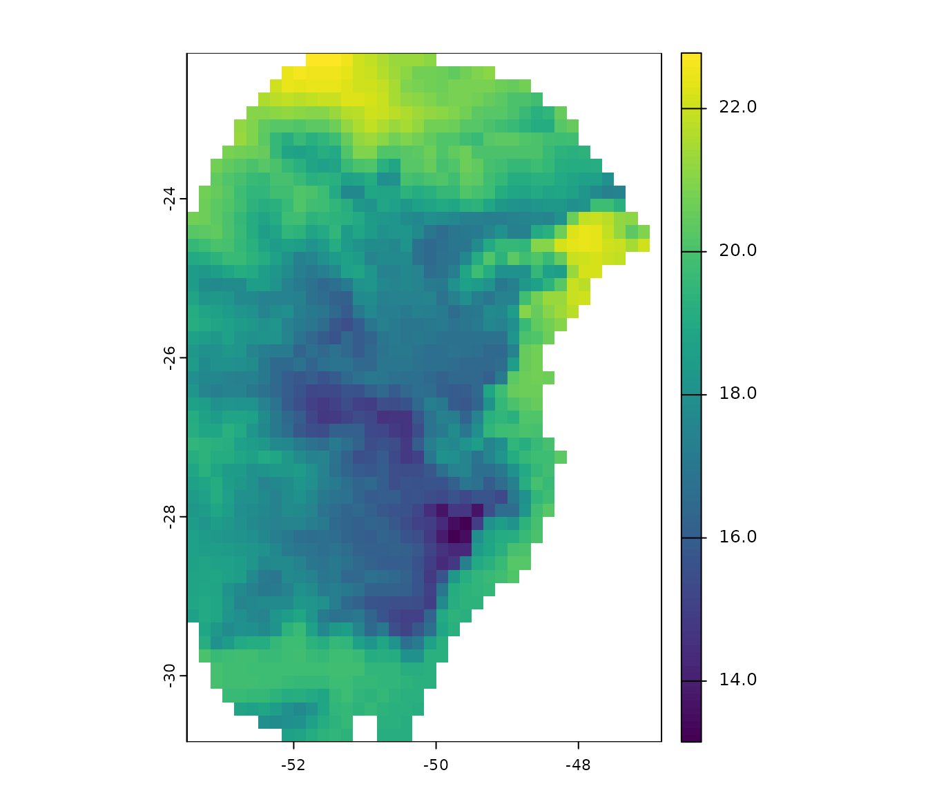
Visualize occurrences records in geography:
# Visualize occurrences on one variable
## Create an extent based on the layer and the records to see all errors
vext <- ext(var)  # extent of layer
pext <- apply(occ_data_noclean[, 2:3], 2, range, na.rm = TRUE)  # extent of records

allext <- ext(c(min(pext[1, 1], vext[1]), max(pext[2, 1], vext[2]),
                min(pext[1, 2], vext[3]), max(pext[2, 2], vext[4]))) + 1

# plotting records on the variable
plot(var, ext = allext, main = "Bio 1")
points(occ_data_noclean[, c("x", "y")])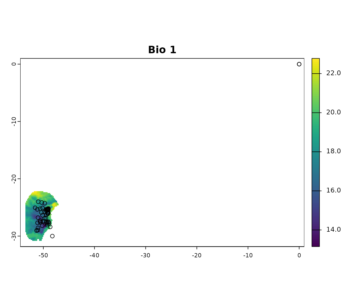
Basic cleaning steps
The basic data cleaning steps implemented in kuenm2 help to: remove missing data, eliminate duplicates, exclude typically (though not always) erroneous coordinates with 0 longitude and 0 latitude, and filter out records with low coordinate precision based on the number of decimal places.
Below is an example of cleaning missing data. This example uses a
data.frame containing only the columns “Species”, “x”, and
“y” (where “x” and “y” represent longitude and latitude, respectively).
If the data.frame includes additional columns and not all
of them should be considered when identifying missing values, users can
specify which columns to use via the columns argument
(default = NULL, which includes all columns). As with any
function, we recommend consulting the documentation for more detailed
explanations (e.g., help(remove_missing)).
# remove missing data
mis <- remove_missing(data = occ_data_noclean, columns = NULL, remove_na = TRUE,
                      remove_empty = TRUE)

# quick check
nrow(occ_data_noclean)
#> [1] 64
nrow(mis)
#> [1] 60
The code below uses the previous results and continues the process of
cleaning data by removing duplicates. The argument columns
can be used as explained before. See full documentation with
help(remove_duplicates).
# remove exact duplicates
mis_dup <- remove_duplicates(data = mis, columns = NULL, keep_all_columns = TRUE)

# quick check
nrow(mis)
#> [1] 60
nrow(mis_dup)
#> [1] 57
Continue the process by removing coordinates with values of 0 (zero)
for longitude and latitude (not always needed, as this location is valid
if working with some marine species). See full documentation with
help(remove_corrdinates_00).
# remove records with 0 for x and y coordinates
mis_dup_00 <- remove_corrdinates_00(data = mis_dup, x = "x", y = "y")

# quick check
nrow(mis_dup)
#> [1] 57
nrow(mis_dup_00)
#> [1] 56
The following lines of code take the previous result and remove
coordinates with low precision. If the longitude and latitude contain no
or only a few decimal places, they may have been rounded, which can be
problematic in some areas. This a step recommended when users know
coordinate rounding is an issue. This filtering process can also be
applied to longitude and latitude independently. See full documentation
with help(filter_decimal_precision).
# remove coordinates with low decimal precision.
mis_dup_00_dec <- filter_decimal_precision(data = mis_dup_00, x = "x", y = "y",
                                           decimal_precision = 2)

# quick check
nrow(mis_dup_00)
#> [1] 56
nrow(mis_dup_00_dec)
#> [1] 51
Users can perform all this steps with a single function as follows:
# all basinc cleaning steps
clean_init <- initial_cleaning(data = occ_data_noclean, species = "species",
                               x = "x", y = "y", remove_na = TRUE,
                               remove_empty = TRUE, remove_duplicates = TRUE,
                               by_decimal_precision = TRUE,
                               decimal_precision = 2)

# quick check
nrow(occ_data_noclean)  # original data
#> [1] 64
nrow(clean_init)  # data after all basic cleaning steps
#> [1] 51

# a final plot to check
par(mfrow = c(2, 2))

## initial data
plot(var, ext = allext, main = "Initial data")
points(occ_data_noclean[, c("x", "y")])

## data after basic cleaning steps
plot(var, ext = allext, main = "After basic cleaning")
points(clean_init[, c("x", "y")])

plot(var, main = "After basic cleaning (zoom)")
points(clean_init[, c("x", "y")])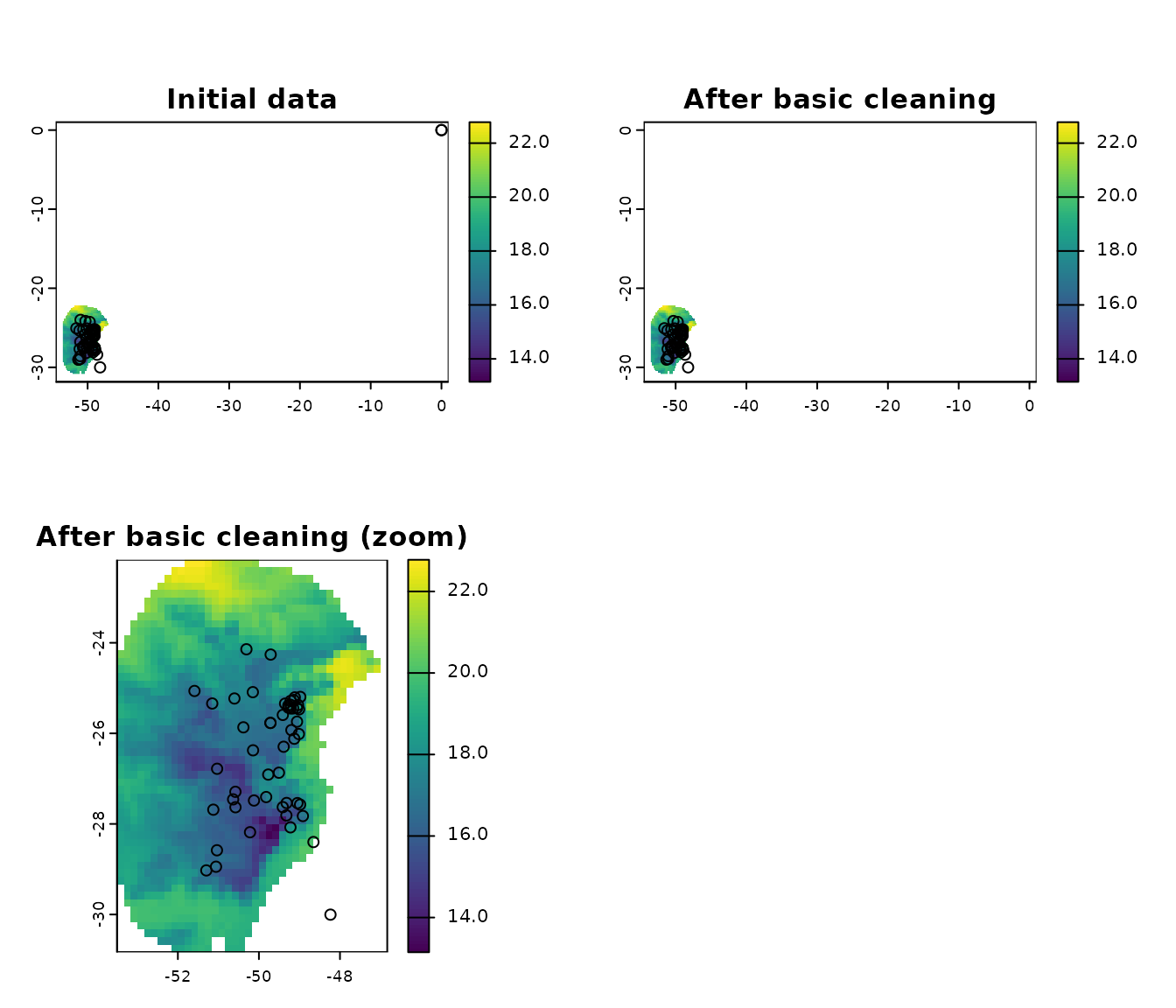
Other cleaning steps
Two additional cleaning steps are implemented in kuenm2, removing cell duplicates and moving points to valid cells.
Removing cell duplicates involves excluding records that are not
exact coordinate duplicates but are located within the same pixel. The
process randomly selects one record from each cell to retain. See full
documentation with help(remove_cell_duplicates).
# exclude duplicates based on raster cell (pixel)
celldup <- remove_cell_duplicates(data = clean_init, x = "x", y = "y",
                                  raster_layer = var)

# quick check
nrow(clean_init)  # data after all basic cleaning steps
#> [1] 51
nrow(celldup)  # plus removing cell duplicates
#> [1] 42
The following lines of code help adjust records that fall just
outside valid raster cells to prevent data loss. Given the nature and
resolution of raster layers, valid records are sometimes perceived as
being outside the boundaries of cells with data. In such cases, an
alternative is to move these records to the nearest valid cell. A
distance limit is applied to avoid relocating records that are too far
from the study area. See below for an example of how to use this
approach. See full documentation with
help(move_2closest_cell).
# move records to valid pixels
moved <- move_2closest_cell(data = celldup, x = "x", y = "y",
                            raster_layer = var, move_limit_distance = 10)
#> Moving occurrences to closest pixels...

# quick check
nrow(celldup)  # basic cleaning and no cell duplicates
#> [1] 42
nrow(moved[moved$condition != "Not_moved", ])  # plus moved to valid cells
#> [1] 41
The function advanced_cleaning facilitates the two processes from above in a single step:
# move records to valid pixels
clean_data <- advanced_cleaning(data = clean_init, x = "x", y = "y",
                                raster_layer = var, cell_duplicates = TRUE,
                                move_points_inside = TRUE,
                                move_limit_distance = 10)
#> Moving occurrences to closest pixels...

# exclude points not moved
clean_data <- clean_data[clean_data$condition != "Not_moved", 1:3]

# quick check
nrow(occ_data_noclean)  # original data
#> [1] 64
nrow(clean_init)  # data after all basic cleaning steps
#> [1] 51
nrow(clean_data)  # data after all basic cleaning steps
#> [1] 41

# a final plot to check
par(mfrow = c(3, 2))

## initial data
plot(var, ext = allext, main = "Initial")
points(occ_data_noclean[, c("x", "y")])

## data after basic cleaning steps
plot(var, ext = allext, main = "Basic cleaning")
points(clean_init[, c("x", "y")])

plot(var, main = "Basic cleaning (zoom)")
points(clean_init[, c("x", "y")])

## data after basic cleaning steps
plot(var, main = "Final data")
points(clean_data[, c("x", "y")])

## zoom to a particular area, initial data
plot(var, xlim = c(-48, -50), ylim = c(-26, -25),  main = "Initial (zoom +)")
points(occ_data_noclean[, c("x", "y")])

## zoom to a particular area, final data
plot(var, xlim = c(-48, -50), ylim = c(-26, -25),  main = "Final (zoom +)")
points(clean_data[, c("x", "y")])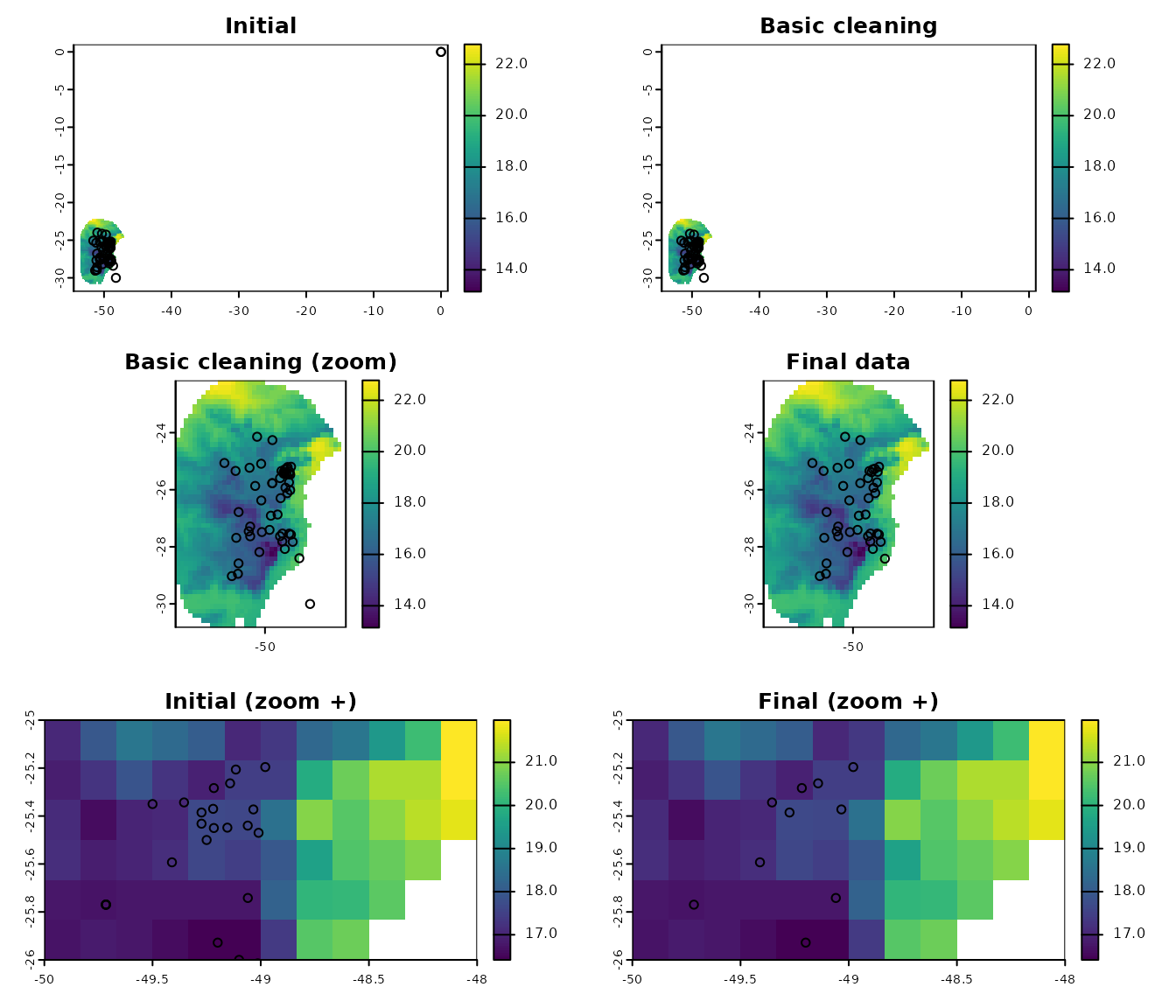
Saving results
The results of the data cleaning steps in kuenm2 are
simple data.frames that may include a few additional
columns and fewer records than the original dataset. An easy way to save
these results is by writing them to CSV files. Although multiple options
exist for saving this type of data, another useful alternative is to
save it as an RDS file in your directory. See the examples below: