Marlon E. Cobos, Vijay Barve, Narayani Barve, Alberto Jimenez-Valverde, and Claudia Nunez-Penichet
- Package description
- Installing the package
-
Using the package functions
- Preparing R
- Simple graphical exploration of your data.
- Species ranges from buffered occurrences
- Species ranges from boundaries
- Species ranges from hull polygons
- Species ranges from ecological niche model outputs
- Species ranges using trend surface analyses
- Nice figures of species ranges
- Species ranges and environmental factors
- Project description

This repository is for the GSoC 2018 project “Species range maps in R” (details at the end).
Package description
The rangemap R package presents various tools to create species range maps based on occurrence data, statistics, and SpatialPolygons objects. Other tools of this package can be used to analyze environmental characteristics of the species ranges and to create high quality figures of these maps. All the functions that create species ranges can also generate representations of species extents of occurrence (using convex hulls) and areas of occupancy according to the IUCN criteria. Shapefiles of the resulting polygons can be saved in the working directory if it is needed.
News
Starting with v 0.1.17, rangemap allows optional calculations of extents of occurrence and areas of occupancy in all main functions (see below). To avoid performing analysies related with these areas, set arguments extent_of_occurrence and area_of_occupancy to FALSE. This change can save time, specially if a large number of occurrences is used.
Installing the package
A stable version of rangemap can be installed from CRAN as follows:
install.packages("rangemap")rangemap can also be installed from its GitHub repository using the following code:
if(!require(remotes)){
    install.packages("remotes")
}

remotes::install_github("marlonecobos/rangemap")
Using the package functions
Preparing R
The following code chunk loads the pacakges needed to perform some example-analyses with rangemap.
The working directory will also be defined in this part.
# working directory
setwd("YOUR/WORKING/DIRECTORY")
Simple graphical exploration of your data.
The rangemap_explore function generates simple figures to visualize species occurrence data in the geographic space before using other functions of this package. The figure created with this function helps to identify countries involved in the species distribution. Other aspects of the species distribution can also be generally checked here; for instance, disjunct distributions, general dimension of the species range, etc.
The function’s help can be consulted using the following line of code:
help(rangemap_explore)An example of the use of this function is written below.
# getting the data
data("occ_d", package = "rangemap")

# simple figure of the species occurrence data
rangemap_explore(occurrences = occ_d)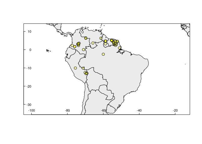
Same figure with country codes.
# simple figure of the species occurrence data
rangemap_explore(occurrences = occ_d, show_countries = TRUE)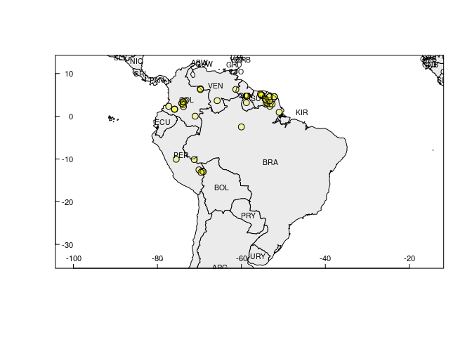
Species ranges from buffered occurrences
The rangemap_buff function generates a distributional range for a given species by buffering provided occurrences using a user-defined distance.
The function’s help can be consulted using the following line of code:
help(rangemap_buffer)An example of how to use this function is written below.
# getting the data
data("occ_p", package = "rangemap")

# species range
buff_range <- rangemap_buffer(occurrences = occ_p, buffer_distance = 100000)

summary(buff_range)
#>
#>                       Summary of sp_range_iucn object
#> ---------------------------------------------------------------------------
#>
#> Species range derived from:  Buffer
#>
#>             Species Unique_records Range_area Extent_of_occurrence
#>  Peltophryne empusa             27   106241.2             66357.71
#>  Area_of_occupancy
#>                 92
#>
#>
#>
#> Other contents:
#>                        Length Class                    Mode
#> species_range           1     SpatialPolygonsDataFrame S4
#> species_unique_records 27     SpatialPointsDataFrame   S4
#> extent_of_occurrence    1     SpatialPolygonsDataFrame S4
#> area_of_occupancy      23     SpatialPolygonsDataFrame S4
The function rangemap_plot generates customizable figures of species range maps using the objects produced by other function of this package. Let’s see how the generated range looks like.
rangemap_plot(buff_range)
For further details see the function documentation.
help(rangemap_plot)Species ranges from boundaries
The rangemap_boundaries function generates a distributional range for a given species by considering all the polygons of administrative entities in which the species has been detected.
The function’s help can be consulted using the following line of code:
help(rangemap_boundaries)Examples of the use of this function with most of its variants are written below.
Using only occurrences
Following there is an example in which administrative areas will be selected using only occurrences. The rangemap_explore function will be used for obtaining a first visualization of the species distributional range.
# occurrence data was obtained in the first example using
# data("occ_d", package = "rangemap")

# checking which countries may be involved in the analysis
rangemap_explore(occurrences = occ_d, show_countries = TRUE)
# getting an example of SpatialPolygonsDataFrame to be used as polygons
data("adm_boundaries", package = "rangemap")

# species range
bound_range <- rangemap_boundaries(occurrences = occ_d, polygons = adm_boundaries)

summary(bound_range)
#>
#>                       Summary of sp_range_iucn object
#> ---------------------------------------------------------------------------
#>
#> Species range derived from:  Boundaries
#>
#>           Species Unique_records Range_area Extent_of_occurrence
#>  Dasypus kappleri             55   12217732              4076154
#>  Area_of_occupancy
#>                176
#>
#>
#>
#> Other contents:
#>                        Length Class                    Mode
#> species_range           7     SpatialPolygonsDataFrame S4
#> species_unique_records 55     SpatialPointsDataFrame   S4
#> extent_of_occurrence    1     SpatialPolygonsDataFrame S4
#> area_of_occupancy      44     SpatialPolygonsDataFrame S4
Figure of the generated range.
rangemap_plot(bound_range)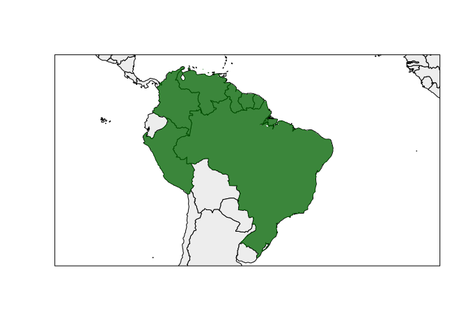
Using only administrative area names
Following there is an example in which administrative areas will be selected using only the names of the administrative entities known to be occupied by the species. This approach may be useful in circumstances where geographic coordinates or accurate locality descriptions do not exist.
# administrative areas invloved
adm <- c("Ecuador", "Peru", "Venezuela", "Colombia", "Brazil")

# species range
bound_range1 <- rangemap_boundaries(adm_areas = adm, polygons = adm_boundaries)

summary(bound_range1)
#>
#>                          Summary of sp_range object
#> ---------------------------------------------------------------------------
#>
#> Species range derived from:  Boundaries
#>
#>  Species Range_area
#>  Species   12043257
#>
#>
#>
#> Species range
#> Object of class SpatialPolygonsDataFrame
#> Coordinates:
#>         min       max
#> x -91.66389 -29.84000
#> y -33.74067  13.37861
#> Is projected: FALSE
#> proj4string : [+proj=longlat +datum=WGS84 +no_defs]
#> Data attributes:
#>   X.Species.           rangekm2
#>  Length:5           Min.   : 255493
#>  Class :character   1st Qu.: 909405
#>  Mode  :character   Median :1135524
#>                     Mean   :2408651
#>                     3rd Qu.:1294369
#>                     Max.   :8448466
Map of the generated range.
rangemap_plot(bound_range1)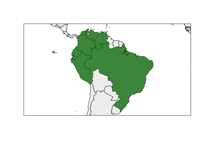
Using occurrences and administrative areas
An example of using both occurrences and administrative areas for creating species ranges with the function rangemap_boundaries is presented below. This option may be useful when these two types of information complement the knowledge of the species distribution.
# other parameters
adm <- "Ecuador" # Athough no record is on this country, we know it is in Ecuador

# species range
bound_range2 <- rangemap_boundaries(occurrences = occ_d, adm_areas = adm,
                                    polygons = adm_boundaries)

summary(bound_range2)
#>
#>                       Summary of sp_range_iucn object
#> ---------------------------------------------------------------------------
#>
#> Species range derived from:  Boundaries
#>
#>           Species Unique_records Range_area Extent_of_occurrence
#>  Dasypus kappleri             55   12473215              4076154
#>  Area_of_occupancy
#>                176
#>
#>
#>
#> Other contents:
#>                        Length Class                    Mode
#> species_range           8     SpatialPolygonsDataFrame S4
#> species_unique_records 55     SpatialPointsDataFrame   S4
#> extent_of_occurrence    1     SpatialPolygonsDataFrame S4
#> area_of_occupancy      44     SpatialPolygonsDataFrame S4
Now the plot.
rangemap_plot(bound_range2)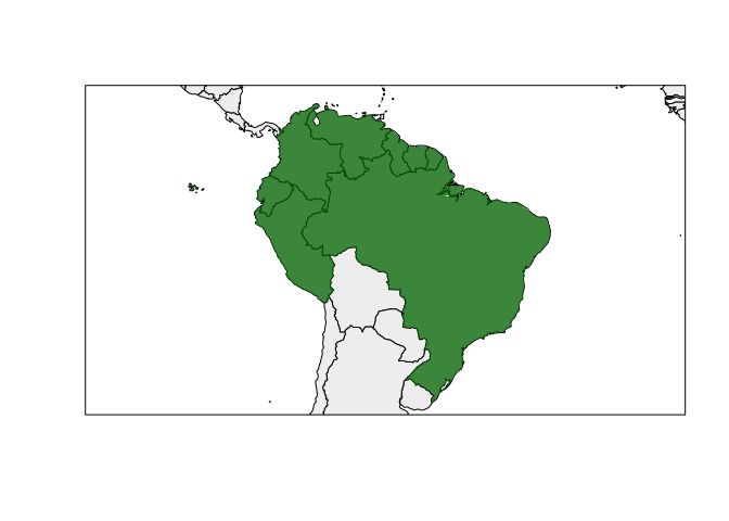
Species ranges from hull polygons
The rangemap_hull function generates a species range polygon by creating convex or concave hull polygons based on occurrence data.
The function’s help can be consulted using the following line of code:
help(rangemap_hull)Examples of the use of this function with most of its variants are written below.
Convex hulls
With the example provided below, a species range will be constructed using convex hulls. After that this range will be split based on two distinct algorithms of clustering: hierarchical and k-means. Convex hull polygons are commonly used to represent species ranges, however in circumstances where biogeographic barriers for the species dispersal exist, concave hulls may be a better option.
# occurrences were obtained in prvious examples using
# data("occ_d", package = "rangemap")

# species range
hull_range <- rangemap_hull(occurrences = occ_d, hull_type = "convex",
                            buffer_distance = 100000)
#> Hull type: convex

summary(hull_range)
#>
#>                       Summary of sp_range_iucn object
#> ---------------------------------------------------------------------------
#>
#> Species range derived from:  Convex_hull
#>
#>           Species Unique_records Range_area Extent_of_occurrence
#>  Dasypus kappleri             56    4860934              4095146
#>  Area_of_occupancy
#>                184
#>
#>
#>
#> Other contents:
#>                        Length Class                    Mode
#> species_range           6     SpatialPolygonsDataFrame S4
#> species_unique_records 56     SpatialPointsDataFrame   S4
#> extent_of_occurrence    1     SpatialPolygonsDataFrame S4
#> area_of_occupancy      46     SpatialPolygonsDataFrame S4


# disjunct distributions
# clustering occurrences with the hierarchical method

# species range
hull_range1 <- rangemap_hull(occurrences = occ_d, hull_type = "convex",
                             buffer_distance = 100000, split = TRUE,
                             cluster_method = "hierarchical",
                             split_distance = 1500000)
#> Clustering method: hierarchical
#> Hull type: convex

summary(hull_range1)
#>
#>                       Summary of sp_range_iucn object
#> ---------------------------------------------------------------------------
#>
#> Species range derived from:  Convex_hull_split
#>
#>           Species Unique_records Range_area Extent_of_occurrence
#>  Dasypus kappleri             56    2115826              4095146
#>  Area_of_occupancy
#>                184
#>
#>
#>
#> Other contents:
#>                        Length Class                    Mode
#> species_range           7     SpatialPolygonsDataFrame S4
#> species_unique_records 56     SpatialPointsDataFrame   S4
#> extent_of_occurrence    1     SpatialPolygonsDataFrame S4
#> area_of_occupancy      46     SpatialPolygonsDataFrame S4


# clustering occurrences with the k-means method

# species range
hull_range2 <- rangemap_hull(occurrences = occ_d, hull_type = "convex",
                             buffer_distance = 100000, split = TRUE,
                             cluster_method = "k-means", n_k_means = 3)

#> Clustering method: k-means
#> Hull type: convex

summary(hull_range2)
#>
#>                       Summary of sp_range_iucn object
#> ---------------------------------------------------------------------------
#>
#> Species range derived from:  Convex_hull_split
#>
#>           Species Unique_records Range_area Extent_of_occurrence
#>  Dasypus kappleri             56    2115826              4095146
#>  Area_of_occupancy
#>                184
#>
#>
#>
#> Other contents:
#>                        Length Class                    Mode
#> species_range           7     SpatialPolygonsDataFrame S4
#> species_unique_records 56     SpatialPointsDataFrame   S4
#> extent_of_occurrence    1     SpatialPolygonsDataFrame S4
#> area_of_occupancy      46     SpatialPolygonsDataFrame S4
Now the figure of the species range.
rangemap_plot(hull_range) # try hull_range1 and hull_range2 as well
Concave hulls
With the following examples, the species range will be constructed using concave hulls. The species range will be calculated as an only area and as disjunct areas by clustering its occurrences using the k-means and hierarchical methods.
# occurrences were obtained in prvious examples using
# data("occ_d", package = "rangemap")

# species range
hull_range3 <- rangemap_hull(occurrences = occ_d, hull_type = "concave",
                             buffer_distance = 100000)
#> Hull type: concave

summary(hull_range3)
#>
#>                       Summary of sp_range_iucn object
#> ---------------------------------------------------------------------------
#>
#> Species range derived from:  Concave_hull
#>
#>           Species Unique_records Range_area Extent_of_occurrence
#>  Dasypus kappleri             56    4327930              4095146
#>  Area_of_occupancy
#>                184
#>
#>
#>
#> Other contents:
#>                        Length Class                    Mode
#> species_range           4     SpatialPolygonsDataFrame S4
#> species_unique_records 56     SpatialPointsDataFrame   S4
#> extent_of_occurrence    1     SpatialPolygonsDataFrame S4
#> area_of_occupancy      46     SpatialPolygonsDataFrame S4


# disjunct distributions
# clustering occurrences with the hierarchical method

# species range
hull_range4 <- rangemap_hull(occurrences = occ_d, hull_type = "concave",
                             buffer_distance = 100000, split = TRUE,
                             cluster_method = "hierarchical",
                             split_distance = 1500000)
#> Clustering method: hierarchical
#> Hull type: concave

summary(hull_range4)
#>
#>                       Summary of sp_range_iucn object
#> ---------------------------------------------------------------------------
#>
#> Species range derived from:  Concave_hull_split
#>
#>           Species Unique_records Range_area Extent_of_occurrence
#>  Dasypus kappleri             56    1878355              4095146
#>  Area_of_occupancy
#>                184
#>
#>
#>
#> Other contents:
#>                        Length Class                    Mode
#> species_range           6     SpatialPolygonsDataFrame S4
#> species_unique_records 56     SpatialPointsDataFrame   S4
#> extent_of_occurrence    1     SpatialPolygonsDataFrame S4
#> area_of_occupancy      46     SpatialPolygonsDataFrame S4


# clustering occurrences with the k-means method

# species range
hull_range5 <- rangemap_hull(occurrences = occ_d, hull_type = "concave",
                             buffer_distance = 100000, split = TRUE,
                             cluster_method = "k-means", n_k_means = 3)
#> Clustering method: k-means
#> Hull type: concave

summary(hull_range5)
#>
#>                       Summary of sp_range_iucn object
#> ---------------------------------------------------------------------------
#>
#> Species range derived from:  Concave_hull_split
#>
#>           Species Unique_records Range_area Extent_of_occurrence
#>  Dasypus kappleri             56    1878355              4095146
#>  Area_of_occupancy
#>                184
#>
#>
#>
#> Other contents:
#>                        Length Class                    Mode
#> species_range           6     SpatialPolygonsDataFrame S4
#> species_unique_records 56     SpatialPointsDataFrame   S4
#> extent_of_occurrence    1     SpatialPolygonsDataFrame S4
#> area_of_occupancy      46     SpatialPolygonsDataFrame S4
Checking the figure.
rangemap_plot(hull_range5) # try hull_range4 and hull_range3 as well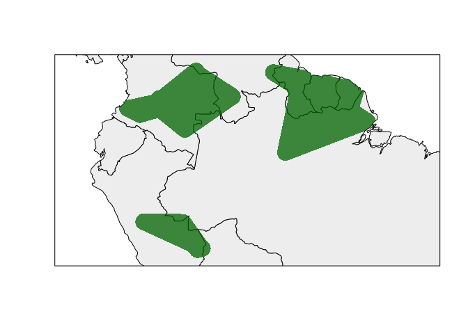
Species ranges from ecological niche model outputs
The rangemap_enm function generates a distributional range for a given species using a continuous raster layer produced with an ecological niche modeling algorithm. This function binarizes the model into suitable and unsuitable areas using a user specified level of omission (a given threshold value).
The function’s help can be consulted using the following line of code:
help(rangemap_enm)An example of the use of this function is written below.
# parameters
sp_mod <- raster::raster(list.files(system.file("extdata", package = "rangemap"),
                                    pattern = "sp_model.tif", full.names = TRUE))
data("occ_train", package = "rangemap")

# species range
enm_range <- rangemap_enm(occurrences = occ_train, model = sp_mod,
                          threshold_omission = 5)

summary(enm_range)
#>
#>                       Summary of sp_range_iucn object
#> ---------------------------------------------------------------------------
#>
#> Species range derived from:  ENM
#>
#>               Species Unique_records Range_area Extent_of_occurrence
#>  Amblyomma_americanum             89    2824883              3535078
#>  Area_of_occupancy
#>                356
#>
#>
#>
#> Other contents:
#>                        Length Class                    Mode
#> species_range          11     SpatialPolygonsDataFrame S4
#> species_unique_records 89     SpatialPointsDataFrame   S4
#> extent_of_occurrence    1     SpatialPolygonsDataFrame S4
#> area_of_occupancy      89     SpatialPolygonsDataFrame S4
Let’s see how this range looks like.
rangemap_plot(enm_range)
Species ranges using trend surface analyses
The rangemap_tsa function generates species range polygons for a given species using a trend surface analysis. Trend surface analysis is a method based on low-order polynomials of spatial coordinates for estimating a regular grid of points from scattered observations. This method assumes that all cells not occupied by occurrences are absences; hence its use depends on the quality of data and the certainty of having or not a complete sampling of the region of interest.
The function’s help can be consulted using the following line of code:
help(rangemap_tsa)An example of the use of this function is written below.
# data
data("occ_f", package = "rangemap")
CU <- simple_wmap("simple", regions = "Cuba")

# species range
tsa_r <- rangemap_tsa(occurrences = occ_f, region_of_interest = CU)

summary(tsa_r)
#>
#>                       Summary of sp_range_iucn object
#> ---------------------------------------------------------------------------
#>
#> Species range derived from:  TSA
#>
#>               Species Unique_records Range_area Extent_of_occurrence
#>  Peltophryne fustiger             18       6825             1630.968
#>  Area_of_occupancy
#>                 48
#>
#>
#>
#> Other contents:
#>                        Length Class                    Mode
#> species_range           1     SpatialPolygonsDataFrame S4
#> species_unique_records 18     SpatialPointsDataFrame   S4
#> extent_of_occurrence    1     SpatialPolygonsDataFrame S4
#> area_of_occupancy      12     SpatialPolygonsDataFrame S4
Let’s take a look at the results.
rangemap_plot(tsa_r, polygons = CU, zoom = 0.5)
Nice figures of species ranges
The rangemap_plot function can be used to plot not only the generated species ranges but also the extent of occurrence and the species records in the same map. The species range will be plot on a simplified world map, but other SpatialPolygons objects can be used.
The function’s help can be consulted using the following line of code:
help(rangemap_plot)Examples of the use of this function are written below.
Including extent of occurrence and species records
rangemap_plot(hull_range5, add_EOO = TRUE, add_occurrences = TRUE)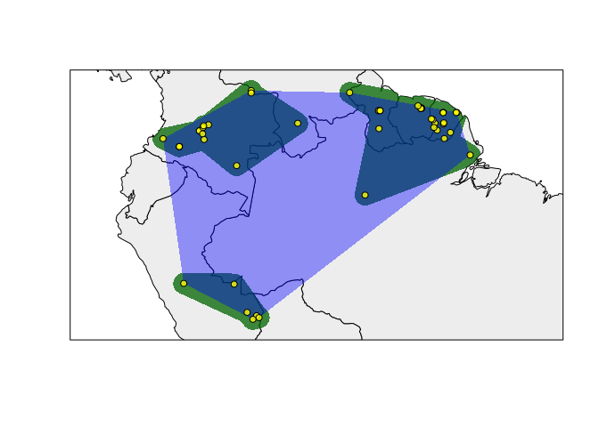
Using other parameters
rangemap_plot(hull_range5, add_EOO = TRUE, add_occurrences = TRUE,
              legend = TRUE, scalebar = TRUE, scalebar_length = 500,
              zoom = 0.5, northarrow = TRUE)
Species ranges and environmental factors
Species ranges on layers of environmental variables
The ranges_emaps function represents one or more ranges of the same species on various maps of environmental factors (e.g. climatic variables) to detect implications of using distinct types of ranges when looking at environmental conditions in the area. Figures can be saved using some of the function’s arguments.
The function’s help can be consulted using the following line of code:
help(ranges_emaps)An example of the use of this function is written below.
# example data
data("buffer_range", package = "rangemap")
data("cxhull_range", package = "rangemap")
data("cvehull_range", package = "rangemap")

vars <- raster::stack(system.file("extdata", "variables.tif",
                                  package = "rangemap"))
names(vars) <- c("bio5", "bio6", "bio13", "bio14")

# plotting
ranges_emaps(buffer_range, cxhull_range, cvehull_range, variables = vars)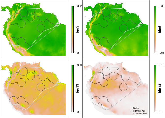
Species ranges in environmental space
The ranges_espace function generates a three dimensional comparison of a species’ ranges created using distinct algorithms, to visualize implications of selecting one of them if environmental conditions are considered.
The function’s help can be consulted using the following line of code:
help(ranges_espace)An example of the use of this function is written below.
# example data
data("buffer_range", package = "rangemap")
data("cxhull_range", package = "rangemap")

vars <- raster::stack(system.file("extdata", "variables.tif",
                                  package = "rangemap"))
names(vars) <- c("bio5", "bio6", "bio13", "bio14")

## comparison
ranges_espace(buffer_range, cxhull_range, variables = vars,
              add_occurrences = TRUE)

# you can zoom in and rotate the figure for understanding it better
Saving this figures for publication can be done using functions from the package rgl (e.g., rgl.postscript() and rgl.snapshot()) .
Project description
Student: Marlon E. Cobos
Mentors: Narayani Barve, Vijay Barve, and Alberto Jimenez Valverde
The species range maps project is motivated by the importance of information about species distribution for processes of conservation planning and the study of spatial patterns of biodiversity. In the face of multiple threats related to Global Change, protection and mitigation actions are crucial for maintaining the health of the planet, and knowing where species are located constitutes in primary information for starting these efforts. Currently, generation of species ranges maps may take several steps and the use of specialized software. Thanks to the recent development of specialized packages, R is rapidly becoming an excellent alternative for analyzing the spatial patterns of biodiversity. Taking advantage of these packages and the versatility of R, the aim of this project was offering handily and robust open source tools to obtain reliable proposals of species distribution ranges and to analyze their geographical patterns. A large community of students, researchers, and conservation managers can be benefited by this project since these tools will be freely available and will improve the way in which studies of species distributions are developed.
Status of the project
A version of the package rangemap (the result of the project) is in CRAN and can be found here.
All commits made can be seen at the complete list of commits.

